Homework 10: Correlation
Objectives:
- Explore null and alternate hypothesis concepts for coefficient estimates and effect size.
- Evaluate error rates (Type I, Type II) and critical value, p-value.
- To compute how to obtain and interpret Product moment correlation and other correlations in R (or R Commander).
Homework 10 expectations
Read through the entire homework before starting to answer a question — all questions are intended to help you achieve the learning outcomes for the chapter. You are expected to have read the chapter and to have completed preceding homework. Answers are provided to odd numbered problems — turn in your work for even numbered problems. A BONUS opportunity is also included.
How to work this homework
This homework includes two datasets, dataset 1 and dataset 2. For BI-311 homework: Answer questions 1 – 4 for dataset 1 and questions 1 – 5 for dataset 2.
Your report will consist of your answers to the bold, numbered questions (both odd and even ones!) and supporting statistics from R. Suggested steps in your analysis are provided as numbered items (regular, not bold format). You may work together or individually, but each of your must turn in your own report. Don’t “plagiarize” from each other. Do include in your report who you worked with.
What to turn in: Turn in one properly named pdf file:
- CORR
The pdfs file contain relevant R code, statistical results — edited to support your answers to the questions, and your answer to the questions (even numbered only). Use of RMarkdown recommended — because it is a simple way to include graphs generated; however copy/paste into a word document is also acceptable.
Note 1: By relevant we mean provide just the R code and results from R functions necessary to support your answers to the questions. For example, do not include
- the entire data set when
head(dataset)will do - screenshots of R output!! R output is text — copy/paste
- all statistical output from an R function.
See Part09: Making a report for an example homework file.
Submit your work to CANVAS. Obey proper file naming formats.
Resources for this homework
Chapter 16. Mike’s Biostatistics Book
Mike’s Workbook for Biostatistics: A quick look at R and R Commander, Part01 – Part10 and previous homework pages presented in this workbook.
Additional R commands and or code provided below.
Work on Correlation
Objective 1: To learn how to obtain and interpret Product moment correlation and other correlations in R and R Commander.
Dataset 1
For correlation analysis, use this dataset = Animals. This data set consists of brain weight and body mass of 28 species, including mammals (24 species plus humans) and three dinosaurs (Brachiosaurus, Dipliodocus, Triceratops). The ratio of brain weight to body mass (brain-body mass ratio) is related to the encephalization quotient (EQ); humans and other primates have a high ratio, so this measure is sometimes taken as a crude estimate of “intelligence.”
Note 2: My description isn’t technically the definition of EQ: see Jerison 1985 and van Schaik et al 2021.
The data set is one of the built-in datasets with R, go to Rcmdr: Data in packages → Read data set from attached package… Select MASS package, then find Animals). Or, just load the data by submitting the code
data(Animals, package="MASS")
Alternatively, for your convenience, I’ve included the dataset at the end of this page (scroll down or click here).
Note 3: Since the 1990s, comparative biologists have recognized that such species comparisons without accounting for phylogenetic structure of the data likely violates the assumption of independence among the data points. Many approaches to account for the nonindependence have been published: see Chapter 20.12 in Mike’s Biostatistics Book for an introduction to one method now called phylogenetically independent contrasts (PIC). For the purposes of this homework we ignore this issue.
Questions for dataset 1: The work to do for correlation analysis
What to do
Use the data provided, and follow the suggested steps 1 – 5, to answer the bold questions below.
1. Make a scatterplot of brain weight on body weight.
a) It would a good idea to highlight specific points in the graph.
Note 4: “… highlight specific points…” This can be done, but it is an advanced R trick (see ggplot2 and gghighlight package). Here’s one method, a bit crude, but it works. Copy and paste the code into the script window of Rcmdr. Assuming you’ve already loaded the dataset Animals, then submit the following code one line a time
classType <- c("M","M","M","M","M","D","M","M","M","M","M","M","M","H","M","D","M","M","M","M","M","M","M","M","M","M","D","M")
dAnimals <-data.frame(classType,Animals)
scatterplot(brain~body | classType, regLine=FALSE, smooth=FALSE, by.groups=TRUE, pch=c(19,19,19), cex=c(2,2,2), col=c("black", "blue", "red"), grid=FALSE, data=dAnimals)
2. Make histograms of body weight and brain weight
3. Conduct a test of normality of brain weight, and another test for body weight
Rcmdr: Statistics → Summaries → Test of normality (Compare Shapiro Wilks against Anderson-Darling)
R code
RcmdrMisc::normalityTest(~body, test="shapiro.test", data=Animals)
4. Obtain the Pearson product moment correlation (parametric) and conduct the two-sided test of the null hypothesis
Rcmdr: Statistics → Summaries → Correlation test
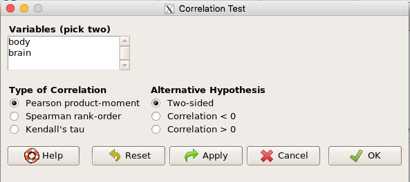
Figure 1. Screenshot correlation test R Commander menu
R code
cor.test(Animalsbrain, alternative="two.sided", method="pearson")
4a. Find in the R output the command for correlation and make sure you include this in your report.
5. Repeat, but this time calculate the (nonparametric) Spearman rank-order correlation, again a two-sided test
5a. Find in the R output the command for Spearman rank-order correlation and make sure you include this in your report.
Question 1. Briefly define and contrast parametric and nonparametric statistical tests. (Hint: assumptions!)
Question 2. Make a preliminary conclusion about whether or not brain weight is correlated with body weight.
Question 3. Using the results from items 2 – 5, which correlation estimate is most justifiable as a test of the association between brain and body weight, the parametric or the nonparametric correlation?
Question 4. Reviewing your plot and the correlation results, comment on the relationship between body mass and brain weight.
Dataset 2
The first dataset reflected a problem routinely addressed in comparative biology. This next dataset touches on an area of biomedical importance, and, has engendered much concern and debate.
You are provided with a data set containing annual values for several variables recorded for birth years beginning in 1992. These include:
- ASD prevalence reported to the CDC per 1000 children.
- Total number of vaccine doses recommended/received by age 2.
- Number of babies named “Michael” by year.
- Number of babies named “Liam” by year.
- Number of licensed acupuncturists in the U.S.
Note 2: Recent surveys suggest about 40% of U.S. women have one or more tattoo.
Tattoo inks can contain many toxins: heavy metals (like lead, mercury, arsenic, cadmium), polycyclic aromatic hydrocarbons (PAHs), and primary aromatic amines (PAAs). These substances are present in both the pigment and solvent portions of the ink (Negi et al 2022).
Because most U.S. states require licensure, but these values are strongly influenced by California, which both requires licensure and has the largest population.
A persistent — but empirically refuted — claim is that vaccines contribute to ASD risk. Proper correlation analysis provides an opportunity to evaluate relationships carefully and recognize when apparent associations are spurious or confounded by other factors.
Note 5: Autism is classified as a neurodevelopmental disorder. As a spectrum disorder, it describes a broad range of neurological and behavioral profiles, reflecting both challenges and strengths, and recognizing that individuals may differ widely in communication, social engagement, learning styles, and sensory experiences. Trends of diagnosed cases have increased significantly over the past decades. Both genetics and environmental factors are associated with ASD. For more, please see Autism Science Foundation. For discussion of “autism and vaccines,” please see their page Autism and Vaccines.
What to do
Use the data provided to answer the bold questions below.
Repeat steps taken above for dataset 1 — you should make appropriate scatter plots and calculate the correlations among the variables.
1. Exploratory Plots
- Create scatterplots of ASD prevalence versus each of the following:
- vaccine doses,
- number of children named Michael,
- number of children named Liam,
- number of licensed acupuncturists.
Question 1: Based on the visual patterns, which variables appear to show a positive or negative association with ASD prevalence? What cautions must you keep in mind when interpreting these plots?
2. Pearson Correlation Coefficients
Calculate the Pearson correlation coefficient between ASD prevalence and each of the four variables.
Question 2: Rank the predictor variables from strongest to weakest correlation with ASD prevalence. Which, if any, appear strongly correlated?
3. Significance vs. Meaningfulness
Question 3: If one or more correlations yield a statistically significant p-value, does that imply a meaningful or causal relationship? Explain why or why not in the context of these particular variables.
4. Interpretation in Public Health Context
Question 4: Based on your analyses, what evidence—if any—supports the claim that vaccine dosing patterns are associated with ASD prevalence? How does your conclusion illustrate the difference between correlation and causation in public health research?
Question 5: How do the correlations involving children’s names or licensed acupuncturists help you evaluate the plausibility of any observed correlation between vaccine doses and ASD prevalence? What does this comparison suggest about interpreting correlations without biological rationale?
Bonus
Jerison’s EQ was calculated as

Calculate and report EQ for chimpanzee, elephant, human, mouse in the Animal data set.
R or Rcmdr commands
myData <- read.table(header=TRUE, sep="\t", text = "
insert your data table here
")

head(myData)
Test normality.
Rcmdr → Statistics → Summaries → Test for normality
Other R/Rcmdr commands provided in text
References
Negi, S., Bala, L., Shukla, S., & Chopra, D. (2022). Tattoo inks are toxicological risks to human health: a systematic review of their ingredients, fate inside skin, toxicity due to polycyclic aromatic hydrocarbons, primary aromatic amines, metals, and overview of regulatory frameworks. Toxicology and Industrial Health, 38(7), 417-434.
Dataset 1
Dataset = Animals from R package MASS
| Animal | body | brain |
|---|---|---|
| Mountain beaver | 1.35 | 8.1 |
| Cow | 465 | 423 |
| Grey wolf | 36.33 | 119.5 |
| Goat | 27.66 | 115 |
| Guinea pig | 1.04 | 5.5 |
| Dipliodocus | 11700 | 50 |
| Asian elephant | 2547 | 4603 |
| Donkey | 187.1 | 419 |
| Horse | 521 | 655 |
| Potar monkey | 10 | 115 |
| Cat | 3.3 | 25.6 |
| Giraffe | 529 | 680 |
| Gorilla | 207 | 406 |
| Human | 62 | 1320 |
| African elephant | 6654 | 5712 |
| Triceratops | 9400 | 70 |
| Rhesus monkey | 6.8 | 179 |
| Kangaroo | 35 | 56 |
| Golden hamster | 0.12 | 1 |
| Mouse | 0.023 | 0.4 |
| Rabbit | 2.5 | 12.1 |
| Sheep | 55.5 | 175 |
| Jaguar | 100 | 157 |
| Chimpanzee | 52.16 | 440 |
| Rat | 0.28 | 1.9 |
| Brachiosaurus | 87000 | 154.5 |
| Mole | 0.122 | 3 |
| Pig | 192 | 180 |
Dataset 2
Dataset collected by Dohm from various sources; ASD Prevalence from CDC, number of children named Michael or Liam from Social Security Administration, vaccine.doses from various CDC and related links, and Acupuncture, which refers to estimated number of licensed practitioners in the U.S.
| Birth | Prevalence | Michael | Liam | Vaccine.doses | Acupuncture |
|---|---|---|---|---|---|
| 2014 | 32.2 | 15496 | 18484 | 29 | 34481 |
| 2012 | 27.6 | 16209 | 16823 | 29 | 30000 |
| 2010 | 23 | 17381 | 10932 | 29 | 28761 |
| 2008 | 18.5 | 20651 | 5980 | 31 | 27965 |
| 2006 | 16.8 | 22651 | 4514 | 31 | |
| 2004 | 14.5 | 25470 | 3827 | 28 | 27663 |
| 2002 | 14.7 | 28158 | 3382 | 28 | |
| 2000 | 11.3 | 32043 | 2781 | 27 | 22671 |
| 1998 | 9 | 36619 | 2209 | 25 | 14228 |
| 1996 | 8 | 38373 | 1748 | 24 | 10623 |
| 1994 | 6.6 | 44475 | 668 | 24 | 8694 |
| 1992 | 6.7 | 54409 | 305 | 24 | 5640 |
/MD