Homework 2A: Descriptive statistics
This homework is about exploring data and is in two parts: this part, Homework 2A, is about Central tendency and Measures of dispersion of data using descriptive (aka summary) statistics. Homework 2B is about data visualization and applies to the same data sets described on this page.
BI311 students: What to turn in
BI-311 students: For homework reports, report only your answers for the even numbered questions; answers to the odd numbered problems are provided to you. Read through the entire homework before starting to answer a question — all questions are intended to help you achieve the learning outcomes for the chapter. It is recommended that you work through the odd numbered problems on your own to confirm your work and as a guide to work the other problems.
Homework 2A expectations
Read through the entire homework before starting to answer a question. All of the coding required was included in Chapter 3 of Mike’s Biostatistics Book. See also relevant tutorials in R work.
How to work this homework
You may work together, but each of your must turn in your own report. Don’t “plagiarize” from each other. Do include in your report who you worked with.
What to turn in: A pdf file containing your answers to the even-numbered questions and relevant R code; by relevant we mean include your code, not copies of code provided to you. For statistical results, report appropriate significant figures. Use of RMarkdown recommended — because it is a simple way to include graphs generated; however copy/paste into a word document, then converted to pdf, is also acceptable.
Note 1: By relevant we mean provide just the R code and results from R functions necessary to support your answers to the questions. For example, do not include
- the entire data set when head(dataset) will do
- screenshots of R output!! R output is text — copy/paste
- all statistical output from an R function.
See Part09: Making a report for an example homework file.
Submit your work to CANVAS. Please obey proper file naming formats.
Resources for this homework
Mike’s Biostatistics Book: Chapter 3
Mike’s Workbook for Biostatistics: A quick look at R and R Commander, Part01 – Part10 and refer also to code presented in Homework 2 from this workbook.
Additional R commands and or code provided below.
Questions
Central tendency
- Find the help page in R for the median function. How does the function handle missing values (NA)?
- For a simple data set like the following
y <- c(1,1,3,6)you should now be able to calculate, by hand, the
• mean
• median
• mode - Confirm your hand calculations from #2.
- If the observations for a ratio scale variable are normally (symmetrically) distributed, which statistic of central tendency is best (eg, less sensitive to outlier values)?
- In Chapter 3 we provided a function to calculate the mode. The function was
temp = table(as.vector(x))names (temp)[temp==max(temp)]In the
names()command, what do you think the result will be if you replacemaxin the command withmin? - If data are not symmetrical, but right skewed — leans to the left, with a tail to the right — will the left to right order of central tendency be
(a) mean equal to the median
(b) mean greater than the median
(c) mean less than the median - Calculate the sample mean and median for the following data sets
(a) Basal 5 hour fasting plasma glucose-to-insulin ratio of one inbred strain of mice, DBA (n = 10, simulated from Table 1 Berglund et al 2008).
x <- c(30.5,48.8, 37.4,56.6,31, 50, 61.2, 74, 63.4, 47.6)
(b) Height in inches of mothers,
mom <- c(67,66.5,64,58.5,68,66.5) #(data from GaltonFamilies in R package HistData)
and fathers,
dad <- c(78.5,75.5,75,75,74,74) #(data from GaltonFamilies in R package HistData)
(c) Carbon dioxide (CO2) readings from Mauna Loa for the month of December for demi-decade 1960 – 2020
years <- c(1960,1965,1970,1975,1980,1985,1990,1995,2000,2005,2010,2015,2020)

#obviously, do not calculate statistics on years; you can use to make a plot
co2 <- c(316.19, 319.42, 325.13, 330.62, 338.29, 346.12, 354.41, 360.82, 396.83, 380.31, 389.99, 402.06, 414.26) #data from Dr. Pieter Tans, NOAA/GML (gml.noaa.gov/ccgg/trends/) and Dr. Ralph Keeling, Scripps Institution of Oceanography (scrippsco2.ucsd.edu/)
(d) Body mass of Rhinella marina (formerly Bufo marinus). Data from M. Dohm,
bufo <- c(71.3, 71.4, 74.1, 85.4, 85.4, 86.6, 97.4, 99.6, 107, 115.7, 135.7, 156.2) - Calculate the sample mean and median for each variable by group.
(a) Body temperature readings, deg C, from IR device on cc body regions (groups). Data from M. Dohm.
body.T <- c(33.2,34.3,34.8,36.1,35.9,35.1,34,34.2,33.6,35.4,35.3,35.4,33.6,33.7,33.8,32.9,34.8,33.7,34.8,33.7,33.1,36.2,34.3,36.3)(b) Distance of darts thrown from bullseye (cm), by two individual dart throwers, aa & bb.
body.R <- c("Forehead","Forehead","Forehead","Throat","Throat","Throat","Forehead","Forehead","Forehead","Throat","Throat","Throat","Forehead","Forehead","Forehead","Throat","Throat","Throat","Forehead","Forehead","Forehead","Throat","Throat","Throat")
dart.D <- c(4.06,8.89,0.00,10.16,11.43,0.00,7.62,7.62,7.37,9.14, NA,10.67)

tossed.by <- c("aa","aa","aa","aa","aa","aa","bb","bb","bb","bb","bb","bb")
(c) Maximum length (cm) on six mollusk species.
shell.length <- c(14.1,17.2,17.6,8,6.83,6.75,6.3,7.7,7.6,6.1,7.2,4.6,17,13.6,13.5,18.5,15.3,19,6.4,7.5,7,7.3,9.1,9)

mollusk.group <- c("SeaStar","SeaStar","SeaStar","Snail","Snail","Snail","SandDollar","SandDollar","SandDollar","Conus","Conus","Conus","Starfish","Starfish","Starfish","Starfish","Starfish","Starfish","Seashell","Seashell","Seashell","Seashell","Seashell","Seashell")
Measures of dispersion
- For a sample data set like
y = c(1,1,3,6), you should now be able to calculate, by hand, the
• range
• standard deviation
• variance - If the difference between Q1 and Q3 is called the interquartile range (IQR), what do we call Q2?
- For our example data set,
x <- c(4,4,4,4,5,6,6,6,7,7,8,8,8,8,8)calculate
• IQR
• sample standard deviation, s
• coefficient of variation - Use the
sample()command in R to draw samples of size 4, 8, and 12 from your example data set stored inx. Repeat the calculations from question 3. For examplex4 <- sample(x,4)will randomly select four observations from x, and will store it in the object x4, like so (your numbers probably will differ!)x4 <- sample(x,4); x4 [1] 8 6 8 6 - Repeat the exercise in question 4 again using different samples of 4, 8, and 12. For example, when I repeat sample(
x,4) a second time I getsample(x,4) [1] 8 4 8 6 - Table 1. Summary statistics mean (+ standard deviation) of height, weight, and waist circumference of 20-39 year old men USA.
Years Height, inches Weight, pounds Waist
Circumference,
inches1999 – 2000 69.4 (0.1) 185.8 (2.0) 37.1 (0.3) 2007 – 2008 69.4 (0.2) 189.9 (2.1) 37.6 (0.3) 2015 – 2016 69.3 (0.1) 196.9 (3.1) 38.7 (0.4) For Table 1, determine how many multiples of the standard deviation for observations greater than 95-percentile (eg, determine the observation value for a person who is in the 95-percentile for Height in the different decades, etc.
- Calculate the sample range, IQR, sample standard deviation, and coefficient of variation for the data sets listed above in question 7 of Central tendency.
- Calculate the sample range, IQR, sample standard deviation, and coefficient of variation for the data sets listed above in question 8 of Central tendency
R commands, copy, paste & modify to Script
To access R help menu for a command, add question mark in front of the command. For example, ?mean brings up the help page in your default browser
IQR()
mean()
quartile()
median()
range()
sample(x, size, replace=FALSE)
sd()
var()
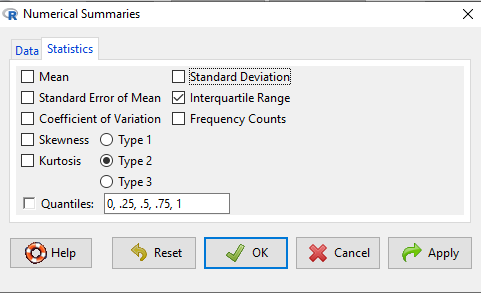
Rcmdr: Statistics → Summaries → Numerical Summaries…, many statistics available in Numerical Summaries
You should pay attention to significant figures. This is a small set of problems with one or two numbers per response, so editing h=by hand probably easiest. However, R has format() command. For example, mean estimate may be 65.08333, but significant figures are just 1 past the decimal.
format(65.08333, 2,3)
returns
65.1