Part 07. Working with your own data
This page is primarily about use of R Commander and local installation of R. However, there are also instructions about R packages that apply to users of R in Google CoLab to import csv and Excel spreadsheet-style files.
Learning objectives
- Import data into R from multiple sources.
- Reshape and enhance datasets within R.
- Use R Commander and base R to streamline data management.
What’s on this page?
- Enter data with combine,
c()- c() vs list()
- Enter data with
scan() - Enter data directly into R with R editor
- Enter data directly within R Commander with R editor
- Reshape a data frame: From unstacked to stacked worksheet
- Add new column (variable) to existing data frame
- Load someone else’s data into R
- text entry
- text (.csv) file
- spreadsheet (
readxlorriopackages) - web scraping from a static webpage (
rvestpackage)
- Enter directly into R
- Load Your Own Data into R from a spreadsheet or CSV file
- Import multiple data files into R
- More practice: Getting your own data into R
- Quiz
What to do
Complete the exercises on this page — judiciously! The goal is for you to find out which method for data entry you prefer, not to work through all of the material here.
Note 1: This page does not cover importing the very large datasets stored in a database. See DBI package used to connect to the database and dbplyr package, which leverages data manipulation using SQL queries directly within the database management system to bring in targeted subsets of data.
The answer depends on how your data is stored. Hint: get in the habit of always storing your data in spreadsheet files, then you only need to learn how to import data from a spreadsheet file — that would be a good choice!
- Create variables with combine
- For small data sets,
scan()may be good option - Enter data directly with R’s Data Editor.
- Enter data directly within R Commander (it’s still R’s Data Editor)
- From unstacked to stacked worksheet in R Commander
- Load someone else’s data into R
- Use
read.table()to enter copied data directly into R - From R, Rcmdr, or Google CoLab, import data from text (.txt, .csv)
- From R, Rcmdr, or Google CoLab, import data from spreadsheet files (Apple Numbers, Microsoft Excel, Google sheets, LibreOffice Calc)
- Save the data file in R format
- Explore simple graphics and statistics with entered data
Note 2: Thus is a very long page, with many twists and turns. Now is an excellent time to remind readers — you only need one way to load your own data into R.
The most straightforward way is to work with csv files — this option requires no additional R packages and is just a matter of pointing R to the file and importing the file via the read.csv() function.
Me? I primarily go with the spreadsheet option because most of my datasets are hundreds to, rarely, thousands of rows. Thus, for small data sets I have my spreadsheet open and I copy and paste the values into a read.table() command. For larger data sets, read.table() would be a poor choice.
Instead, I usereadxl. These commands work across R environments, from local installs to Google CoLab. The R package openxlsx is more capable than readxl; in addition to reading Excel files, openxlsx permits writing to and editng excel files. I don’t discuss use of openxlsx further.
The package rio may be your best option. It simplifies data import and export, capable of detecting csv, ods, or xls and xlsx files, although in the case of ods, xls, or xlsx files, rio is a wrapper function to the readODS, readxl, and openxlsx packages, respectively. Thus, you’d need to have those packages installed before use of rio.
How to do it
For these exercises, you may work
- within the Rcmdr script window.
- at the command line and R prompt.
- from a script document and the R GUI app.
- RStudio.
- Google CoLab or other cloud service.
Choose one way. If you’re working with R on your computer, then the quickest way is to just work with R Commander. or create a new script document to run in the R app. If you are working with Google CoLab, the instructions presented here apply with minimal changes required.
CoLab users — as a reminder, you may need to install and load additional packages to carry out exercises, given that the instructions assume use of R Commander, and therefore, the described packages would already be loaded and available to the user. Installing packages was detailed in the previous tutorial page, Part 05. R packages: Making R do more.
Let’s begin.
Before you start
A reminder, always set your working directory in R first (see Part 02. Getting started with R and Rcmdr), before starting to do your analyses. Makes life a lot easier.
As you may imagine, data may come from a variety of sources and R-project has detailed instructions to cover many situations (R Data Import/Export manual). The following discussion covers situations common to BI311 and other beginning statistics courses.
Google CoLab users — we assume you have mounted your Google MyDrive and all scripts and personal datasets are available in MyDrive.
1. Enter data with combine
The function c() is useful for entering small sets of numbers or other elements, as long as they are the same type (atomic vectors).
Geckos <- c(3.186, 2.427,4.031,1.995)
Anoles <- c(5.515,5.659,6.739,3.184)
Then, create your data frame.
lizard <- data.frame(Geckos,Anoles); lizard
Output from R
 Geckos Anoles
1 3.186 5.515
2 2.427 5.659
3 4.031 6.739
4 1.995 3.184
Note 2: This data format is termed an unstacked or wide format. More often we need a stacked worksheet, like so:
  Spp Mass
1 Geckos 3.186
2 Geckos 2.427
3 Geckos 4.031
4 Geckos 1.995
5 Anoles 5.515
6 Anoles 5.659
7 Anoles 6.739
8 Anoles 3.184
This is a simple data set so easy enough to create using a read.table() call (see below).
c() vs list()
Alternatively, we might want to create it as data.frame as follows:
lizards <- data.frame("Geckos", "Anoles")
lizards$Geckos <- c(3.186, 2.427, 4.031, 1.995)
lizards$Anoles <- c(5.515, 5.659, 6.739, 3.184)
However, when running the code you’ll find that the lizards data.frame remains empty and R reports with [8] ERROR: replacement has 4 rows, data has 1.
Note 3: A data.frame in R is a type of object used to store data in a table format. A data.frame is like a spreadsheet. Think rows and columns, with columns often used to contain variables, and rows pointing to observations on a sample.
Instead, create a list, add the variables to the list and then convert the list to a data.frame (h/t conversation at stackoverflow.com).
myList <- list(Spp = NA, Mass = NA)
l1 <- "Geckos"; l2 <- "Anoles"
Spp <- c(rep(l1,4), rep(l2,4))
Mass <- c(3.186, 2.427, 4.031, 1.995, 5.515, 5.659, 6.739, 3.184)
myList$Spp <- Spp
myList$Mass <- Mass
lizards <- as.data.frame(myList)
Both c() and list() look very similar, the difference is that list() is more general — you can create a vector of mixed types. c()
Note 4: The trick with rep(). Instead of repeatedly typing “Gecko” and “Anoles” four times each, we used rep() which is short for repeat.
Variants
You may need to create a variable with repeated elements. For example, I need a variable (a factor variable, actually), that marks time points in minutes, from zero to ten, and I need it to repeat for n = 3 trials. Here are two possible methods.
myT <- c(0:10)
newT <- rep(myT, each=3)
Print newT and R returns
 [1] 0 0 0 1 1 1 2 2 2 3 3 3 4 4 4 5 5 5 6 6 6 7 7 7 8
[26] 8 8 9 9 9 10 10 10
The second method repeats the sequence in order
repT <- rep(myT, times=3)
and R returns
 [1] 0 1 2 3 4 5 6 7 8 9 10 0 1 2 3 4 5 6 7 8 9 10 0 1 2
[26] 3 4 5 6 7 8 9 10
Note 5: A factor variable is a categorical variable (see Chapter 3.1 – Data types), which can be either numeric or character string. Many R functions work best if categorical variables are declared as factor variables, factor() or as.factor().
I may want to print the elements of a vector one per line.
cat(repT,sep="\n")
where cat is short for concatenate will do just that. Concatenate is an operation in computer languages to put strings of characters together; "\n" instructs to start characters on new lines.
2. Enter data with scan()
CoLab, skip this step.
Again, for small data sets, a good option may be scan() — simply type in your numbers to objects.
gecko <- scan()
After typing the code, then pressing theEnter key, you will be prompted to enter your numbers one at a time. An in-progress use of scan() is displayed below.
1: 3.186
2:
Enter the four numbers, then follow with another return to end the entry. Repeat for the next variable, anoles. Create a data.frame as above to complete the data entry.
3. Enter data directly into R
CoLab, skip this step.
Base R has a simple editor, Data Editor, that you can call to enter data into a spreadsheet-like form. First, create the data.frame object. “Everything in R is an object.”
myData <- data.frame()
Second, call the editor
myData <- edit(myData)
You should see the Data Editor form (Fig 1).
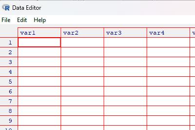
Figure 1. Screenshot of R’s simple Data Editor.
Begin data entry. For an example, Table 1.
Table 1. Color and weights (g) of 16 M&M’s®
| Color | Mass |
|---|---|
| Orange | 0.80 |
| Orange | 0.81 |
| Orange | 0.80 |
| Orange | 0.85 |
| Orange | 0.84 |
| Orange | 0.77 |
| Orange | 0.83 |
| Orange | 0.87 |
| Blue | 0.83 |
| Blue | 0.87 |
| Blue | 0.83 |
| Blue | 0.91 |
| Green | 0.86 |
| Brown | 0.87 |
| Red | 0.79 |
| Red | 1.11 |
click on var1 in the header row, enter the variable name Color, select character, then return (Fig 2).
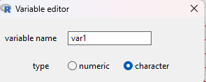
Figure 2. Screenshot variable editor form.
Repeat entry of variable names. Select numeric for Mass. To enter data, click in the first cell and enter the value. Use keyboard arrow keys, or mouse pointer to move between cells. Figure 3 shows a few entries in the Data Editor.
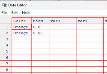
Figure 3. Screenshot data entry in R Data Editor.
To view the data, type myData (or whatever you named the object) at the R prompt. R returns
> myData
   Color Mass
1 Orange 0.80
2 Orange 0.81
>
4. Enter data directly within R Commander.
CoLab, skip this step.
If you haven’t already, start R Commander
library(Rcmdr)
To open a new worksheet in Rcmdr — it’s still R’s Data Editor — follow these steps.
Data → New data set…
then enter a name for the data set, e.g., lizards, in the pop-up dialog box and click OK to continue.
Change the default variable names to “gecko” in Var1 and “anoles” in Var2. Hint: To change the variable name, click on the column and a new popup menu will appear. Change the variable name from Var1 to “gecko”
Enter the data and labels stacked into columns, with row one enter”3.186″ in “gecko” (Var1) and “5.515” in “anoles” (Var2), without the quotes, of course. After you are done, you have an unstacked worksheet, which should look like (Fig 3).
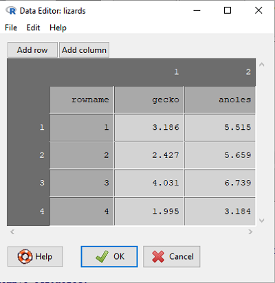
Figure 3. Screenshot of R worksheet editor view.
To finish the worksheet select
File → Close
5. Reshape a data frame: From unstacked to stacked worksheet.
The format of lizards, the data set we just created above, is in wide format aka an unstacked worksheet (row to column orientation). In most cases I am aware of, R expects your data in long form, also known as a stacked worksheet (column to row orientation) because most statistical functions in R expect that format.
Question 1: True or False. We can use the R editor to create a stacked (wide) data set instead of an unstacked (long) worksheet.
Answer. True, of course!
In R, we can reshape the unstacked data frame with stack(). Assume an unstacked data.frame, like the one we entered in Note 2 above. The data frames was stored in the object lizard.
# Stack and save to new data frame
df <- stack(lizard)
We need to rename the variables after stacking. Check
names(df)
R returns
[1] "values" "ind"
We could go with those unhelpful default variable names, but in keeping with good data management principles, we will replace with more appropriate column names.
The following code replaces the variable names
names(df)[names(df) == "values"] <- "mass"
names(df)[names(df) == "ind"] <- "lizard"
Check your work by running names() again.
names(df)
now returns
[1] "mass" "lizard"
If more than one variable name needs changing, an alternative to one-at-a-time approach described above is setNames().
df <- setNames(df, c("mass","lizard")
will do the trick.
CoLab, skip this step. R Commander. It is easy to go from unstacked to stacked in Rcmdr. This process is referred to as reshaping the data frame.
Data → Active data set → Stack variables in active data set…
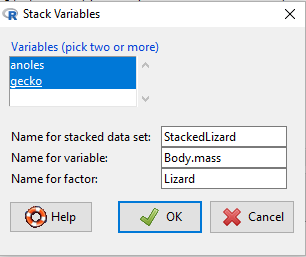
Figure 4. Screenshot of filled out Stack variables menu
You can confirm that your data entry is saved correctly by clicking on the View data set button (Fig 5).
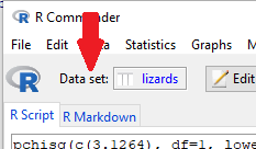
Figure 3. Screenshot of Rcmdr, red arrow points to Data set button.
Click on the button to bring up popup menu shown in Figure 4.
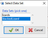
Figure 4. Select the new data set.
6. Add new column (variable) to existing data frame
If we need to add a variable to an existing data frame, the new variable must have the same length. For example, add IDs 1 – 4 for geckos and 1 – 4 for anoles lizards in the data frame df. Use the rep() command we introduced before.
myID <- c(1:4)
myIDs <- rep(myID, times=2)
Use the $ operator
df$ID <- myIDs
Check results, print df, R returns
   mass lizard ID
1 3.186  gecko  1
2 2.427  gecko  2
3 4.031  gecko  3
4 1.995  gecko  4
5 5.515 anoles  1
6 5.659 anoles  2
7 6.739 anoles  3
8 3.184 anoles  4
which is what we expect.
Note 6: The first column is called the index column, 1 – 8 without a header, is part of the data frame structure set by R. You can hide the index row by print(df, row.names=FALSE)
Although unnecessary, I would reorder the variables. Simple way is to recognize that column order in df is mass is column 1, lizard is column 2, and ID is column 3. Therefore,
df2 <- df[, c(3, 2, 1)]
and check the results
 ID lizard  mass
1 1  gecko 3.186
2 2  gecko 2.427
3 3  gecko 4.031
4 4  gecko 1.995
5 1 anoles 5.515
6 2 anoles 5.659
7 3 anoles 6.739
8 4 anoles 3.184
And recall that the comma in [, c(3,2,1)]? That tells R to collect all rows from the data frame.
7. Load someone else’s data into R
A frequent operation in data analysis is the need to access and load data from a remote source. This is called “web scraping,” among many other terms to describe this behavior (see web scraping from a static webpage (rvest package). We’ll use a simple technique called copy and paste. We’ll go over a couple of options, one is to create a text file and then use R to manipulate the data into the format we need. Another option is to use a spreadsheet program instead — since most of you will be more comfortable with the spreadsheet software, this may be the preferred method for you. You should try both! The data we want to get into R are displayed in Table 2.
Table 2. Miles per hour for a 19.7 mile morning commute by Chevy S-10 on Oahu over eight consecutive weeks (2011).
| Monday | Tuesday | Wednesday | Thursday | Friday |
|---|---|---|---|---|
| 38.323 | 40.966 | 39.6 | 45.692 | 39.6 |
| 34.941 | 31.263 | 36 | 42.429 | 36 |
| 36 | 32.108 | 28.286 | 37.125 | |
| 32.108 | 28.286 | 26.4 | 28.976 | 40.966 |
| 47.52 | 36 | 33 | 32.108 | 31.263 |
| 42.429 | 39.6 | 36 | 38.323 | 39.6 |
| 38.323 | 38.323 | 30.462 | ||
| 23.294 | 31.263 | 31.263 | 31.263 | 24.75 |
8. Enter data directly into R.
Section 8 is a long passage, with many twists and turns. Now is an excellent time to remind readers — you only need one way to load your own data into R.
Me? I primarily go with the spreadsheet option because most of my datasets are hundreds to, rarely, thousands of rows. Thus, for small data sets I have my spreadsheet open and I copy and paste the values into a read.table() command. For larger data sets, read.table() would be a poor choice. Instead, I usereadxl.
For small data sets, you can paste the data set between text="", use
myTable <- read.table(header=TRUE, sep="\t", fill=TRUE, text="")
at the R prompt, where the columns are separated by tabs use sep="\t"(if separated by a single space, use sep=""), fill=TRUE is used to fill the empty space, missing values, from our table, and you would paste the scraped table or copied table from your spreadsheet (see Load Your Own Data into R), between the double quotes following text="". The result will be an object stored in R as a data frame, ready for your work.
Note 7. Column separated values on webpages picked up by copy/paste can be inconsistent. The best advice is to view the page contents and confirm, but a bit of trial and error will also solve it. First, assume tabs and try sep="\". If this fails, try a single space, sep="".
For an example, I copied all data rows and the header row from Table 1, then pasted between the “” at the R prompt, although it would be easier if you pasted the text into R script, then run the command from your script (macOS: Cmd + Enter; Win11: Ctrl + R).
Here’s results of copy
myTable1 <- read.table(header=TRUE, sep=" ", fill=TRUE, text="
Monday Tuesday Wednesday Thursday Friday
38.323 40.966 39.600 45.692 39.600
34.941 31.263 36.000 42.429 36.000
36 32.108 28.286 37.125 40.966
32.108 28.286 26.4 28.976
47.52 36 33 32.108 31.263
42.429 39.6 36 38.323 39.6
38.323 38.323 30.462
23.294 31.263 31.263 31.263 24.75
")
Note 8. With respect to missing values. R seems to handle missing values best if you specify the missing value as NA instead of blank in your data set. Add na.strings = "NA" in place of fill=TRUE.
Verify the import, used head() function, which grabs the first six rows (or, tail() function, which grabs last six rows).
> head(myTable1, 3)
Monday Tuesday Wednesday Thursday Friday
1 38.323 40.966 39.600 45.692 39.600
2 34.941 31.263 36.000 42.429 36.000
3 36.000 32.108 28.286 37.125 40.966
Note 9. I entered “3” in head(), which restricts the command to return the first three rows only.
Working with text files is more robust approach than copy/paste into your R script.
Highlight and then copy the table into your clipboard.
- You can Open your text editor (e.g., TextEdit on a macOS; Notepad on Windows) and paste the contents into the blank text page.
For example, I saved the table to a file calledmytable.txtin my working folder. - Or, and this is the quickest (but may fail!) — once you’ve copied the table, it is now in the Clipboard, so R Commander has an option to retrieve from your clipboard, proceed directly to R Commander/Clipboard option described below.
Note 10: macOS users — if copy/paste fails with R, see Can’t copy/paste into R script, macOS to solve the problem.
Replace text="" with file="" in the read.table() function. The code now is
myTable <- read.table(header=TRUE, sep="\t", fill=TRUE, file="myTable.txt")
For larger data sets, data may be imported as a text file, commonly one where variables (columns) are separated by commas. you can paste the data set between text="", use
myTable <- read.table(file.choose(), header=TRUE, sep=",")
or, if you know the name of the file, replace file.choose() with the name of the file in quotes, e.g., "myData.csv".
Do on your own. Copy and paste the data below into your text editor, save the file as .txt or .csv, then load the data in R and save to data frame object of your choosing.
Monday,Tuesday,Wednesday,Thursday,Friday
38.323,40.966,39.600,45.692,39.600
34.941,31.263,36.000,42.429,36.000
36,32.108,28.286,37.125,40.966
32.108,28.286,26.4,28.976,NA
47.52,36,33,32.108,31.263
42.429,39.6,36,38.323,39.6
38.323,38.323,30.462,NA,NA
23.294,31.263,31.263,31.263,24.75
Note “NA” added to denote missing value.
Web scraping from a static webpage (rvest package)
In Part 03. Explore use of R, we copied data from a table and imported it into an R data frame via read.table(). Here, we’ll introduce R’s capabilities to grab data directly from a web page. Mike’s Workbook for Biostatistics and Mike’s Biostatistics Book are presented as static web pages (Wikipedia); it’s relatively straightforward to grab data from my sites. The following code will scrape and return the table data into a data frame object, ready for use.
Download and install rvest package, which is part of the larger tidyverse package for data science produces by Hadley Wickham and friends. We’ll just install rvest, but by installing tidyverse, you get rvest and many other useful tools that make R work even better. Because there’s only the one table on the page, only two commands are needed: we read the web page and save it to an object, then call for the table with the html_table() function.
library(rvest)
webPage <- read_html("https://mikeworkbook.letgen.org/r-work/a-quick-look-at-r-and-r-commander/part-03-explore-use-of-r/")
myWeb <- as.data.frame(html_table(webPage))
Note 11: If you copy entire table from the web page, and you include column headers in first row, then html_table(webPage, header=TRUE). Alternatively, skip the header row, copy only the data, and leave as the default html_table(webPage). The columns will be assigned names like V1, V2, etc. You can then rename the header row, as we described above in Reshape a data frame: From unstacked to stacked worksheet.
#Check the import
head(myWeb)
and R returns
 Min Trial01 Trial02 Trial03 Trial04
1 0 82.8 88.7 83.2 86.2
2 1 76.7 78.5 77.6 NA
3 2 69.4 74.3 72.5 74.3
4 3 67.2 71.4 70.7 68.9
5 4 63.3 67.6 68.5 61.5
6 5 60.6 65.5 65.8 57.7
That was easy!
rvest returns tibbles because the tidyverse world uses tibbles. Tibbles are more flexible than a data frame, but to be consistent with the rest of our work, we stick to data frames. If you want to know more about “tibble,” feel free to do a query, “why is it called tibble?”
Note 12: By sharing web scraping code, and pointing y’all to my web site, I give my permission for readers to web scrape data from Mike’s Biostatistics Book and Mike’s Workbook for Biostatistics. However, don’t abuse the gift. First, the data are copy right protected, albeit with a Creative Commons license. Second, don’t hammer my — or especially other’s — websites with excessive web scraping activity, which can harm the performance of a web site or even violate the rules of the hosting service for the website. Third, be aware and apply web scraping etiquette, e.g., see 2020 post by Alexandra Datsenko at Webbiquity. For other sites, be advised that you would be wise to review their conditions of use or terms of service statements before proceeding to scrape their pages. LinkedIN, for example, prohibits “… scrap[ing] the Services or otherwise copy profiles and other data from [LinkedIN].”
R Commander
CoLab, skip this step.
Text file option
- Return to R Commander and select Data → Import data → from text file, clipboard, or URL…
- Enter a name for the data set, e.g.,
myData - Location of data file:
- If you are loading from a text file, then check Local file system (Figure 5)
- If you are loading directly from the clipboard, then check Clipboard (Figure 6)
- Field separator: check “Tabs”
- Leave the rest as default values
- Click OK
- Enter a name for the data set, e.g.,
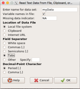
Figure 5. Rcmdr load data from a text file from Local file system.
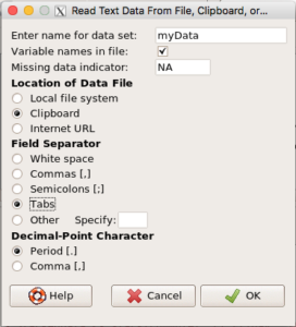
Figure 6. Rcmdr load data from Clipboard.
- Now, the dataset should be loaded in R. Check the Message window in R to see if there were errors.
- We need to convert the dataset into a long, stacked format. This is easy to do in Rcmdr.
- Data → Active data set → Stack variables in active data set…
- Select the columns (variables), enter a new name for the stacked data set, enter name for the data variable (
mph), and a name for the factor (DaysOfWeek), see Figure 7.
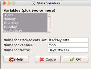
Figure 7. Rcmdr stack data from an unstacked (wide) data set.
Spreadsheet option
- Now, please open your spreadsheet app (e.g., Google Sheets, MS Excel), then return to this page and highlight/copy the data table to your clipboard.
- Return to Excel and paste the data into a worksheet.
- Convert the stacked worksheet into a stacked worksheet (see Hint below).
- In your Excel file, stack the data into two columns (long form).
- Label the first column “
DaysOfWeek” and the second column “mph” (without the quotes).
- Save the workbook and remember where on your computer you saved the file.
- Next, upload the data file to R from within R Commander
- Data → Import data → From Excel file
- Select the correct worksheet from the popup menu.
- Data → Import data → From Excel file
Screenshot of an unstacked or wide format data set based on the data from Table 1 is displayed in Figure 8. See Figure 9 for a stacked (long format) version of the same data set as in Figure 8.
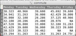
Figure 8. Screenshot of an unstacked or wide format worksheet
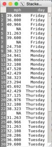
Figure 9. Stacked or long format worksheet
Save the data file in R format
Finally, save the data you imported as an R file (.RData)
- Data → Active data set → Save active data set…
- Save the file with an appropriate file name to your working folder (Figure 10)
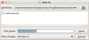
Figure 10. Rcmdr Save As popup dialog.
Question 2. Try each of the three ways to get Table 1 data into R: Clipboard, text file, spreadsheet file.
Question 3. Once the data set is loaded in R, find the missing value(s) for the dataset. Report the row number(s) for the missing value(s).
Hint: Use is.na() function. Just enter the name of the variable to check for missing value(s). This will return a vector with FALSE for each non missing case, and TRUE for any missing value. Quick-R website provides this set of commands which you should also try
dataset[!complete.cases(dataset),]
where “dataset” is replaced with the name of your data set loaded in R. Try both!
Question 4. What kind of graph would be suitable to display the relationship (if any) between DaysOfWeek and mph? Explore the available default graphs in Rcmdr and select one.
A) bar chart
B) histogram
C) pie chart
D) scatter plot
Note 13: Question 3 and 4 are part of Part 08. Data exploration. You should open and work through Part 08, then return to complete or expand on your investigation of Question 3 and 4.
Data import into R (Rcmdr)
Work with one table at a time. R can handle multiple data sets in memory, but you work with one data set a at a time. You have several options — select the one that works best for you.
- In your browser, highlight and copy the table (skip the table label — just the column header and numbers), then, in R go to Rcmdr: Data → Import data → from text file, clipboard, look for any error messages, then check data by “View data” button.
- If the copy-paste from clipboard method fails for you, then copy and paste the data into an Excel spreadsheet. Then, import the data from a saved Excel spreadsheet in R by Rcmdr → Data → Import data → From excel file, look for error messages, then check data by “View data” button (only available if you are working with Rcmdr version 2.04 or higher — all of the NSM Macbooks should meet this requirement).
- After entering the data into Excel, export the data from your Excel spreadsheet as a text file. Then, import the data into R by Rcmdr → Import data from text file, look for error messages, then check data by “View data” button. If you do not know how to export to text file, please check our Moodle help pages.
Regardless of the approach you used, once you get the data into R, save the data in R format before proceeding. Rcmdr: Data → Active data set → Save active data set
I want you to either work with text files you create or Excel files you create, hence this exercise. This becomes important later in the course when you work with your own datasets. However, I will provide you with an Excel file with the two datasets (Knell, RalphPearson) just in case you run into trouble with data loading so that you’ll be able to move onto the descriptive statistics and graphics. Click here to get the RWork01.
9. Load Your Own Data into R from a spreadsheet or csv file.
This section describes how to import data in the form of Microsoft Excel style (xls or xlsx) spreadsheet files of comma separated values text file (txt or csv). Instructions primarily apply to local R installation, but include also how to import files in Google CoLab running R.
Think about your other science classes. Do you have data? It may be as simple as data for a calibration curve or a set of data for growth rates of a cell line. At a minimum, you will generate data for your research projects. As we proceed with projects, bring these data sets into R by either the text file route or the spreadsheet route.
Loading csv data files into R requires no aadditional packages. Thus, one option is to convert any spreadsheet file to csv, then to import the text file into R. See this page for instructions how to save a spreadsheet file — Apple Numbers, Google Sheets, LibreOffice Calc, Microsoft Excel — at Spreadsheets and data entry.
Local R installation
Loading a data file into a local installation of R or into Google CoLab running R will be different because of differences in file access. However, the read.csv() function is used in either case.
In a local R environment, assign the data to a variable named my_data or any other valid named R object. Then choose among the following options
Option 1: the file is located in the active R working directory.
my_data <- read.csv("datafile.csv")
Option 2: specify the path to the file
my_data <- read.csv("C:/Users/YourUsername/Documents/datafile.csv")
Option 3: use a second function, file_choose(), to navigate to and select the file
my_data <- read.csv(file_choose())
In all cases, I recommend checking that the data.frame was created successfully (head()), and attaching the data.frame (attach(my_data)), so that variables are easily referenced in R code.
Google CoLab
If running R in Google CoLab, then the notebook runs in the cloud, so you cannot directly access a file by pointing to your computer’s local file path. Option 1: upload the file to the Colab environment via a Python command — which means the file will only be available for the current session, or Option 2: connect your Google Drive. This allows R to access files stored in your Google Drive and therefore available over different sessions. This option also requires use of a Python command.
Note 14. These code snippets were drawn from AI Gemini, from conversations in Stack Overflow, with code and descriptions modified for consistency and clarity to fit the page style.
Option 1: Session only access. Run a Python command to enable file upload
cat(system('python3 -c "from google.colab import files;
    uploaded = files.upload()"',
    intern=TRUE), sep='\n', wait=TRUE)
After running this command, you can load it into R.
my_data <- read.csv("datafile.csv")
Option 2: Connect Google drive. Run a Python command to mount Google Drive.
cat(system('python3 -c "from google.colab import drive;
    drive.mount(\'/content/drive\')"',
    intern=TRUE), sep='\n', wait=TRUE)
This command will create a url link; click the link, authenticate your account, then copy and paste the verification code into the input box in the Colab output.
Next, replace path/to/your/datafile.csv with the actual path.
my_data <- read.csv("/content/drive/My Drive/path/to/your/datafile.csv")
Again, confirm that the data.frame was created successfully (head()), and attaching the data.frame (attach(my_data)), so that variables are easily referenced in R code.
Loading spreadsheet data files into R from a spreadsheet app is a common task to accomplish. Microsoft Excel is the most popular spreadsheet app, and there are several R packages dedicated to working with Excel files. So, if using Apple Numbers, Google Sheets, or LibreOffice Calc, one options is to export your file into an Excel supported file (xls or xlsx) — see Spreadsheets and data entry.
Note 15: Instead of sheet number, can point to the sheet by name, e.g., sheet = "Sheet2".
The are packages dedicated to work with Google Sheets,googlesheets4 package, details discussed below.
Alternatively, the ods — OpenDocument spreadsheet — format default in LibreOffice Calc (readODS package), but discussion on this pformat is not presented here.
There appears to be no R packaged specialized to handle the proprietary Apple Numbers file format. Thus, if Numbers file, then best option is to export the file as csv as described above.
This page describes two packages that help import Excel files,readxl and rio. We assume that you have already installed the packages via the usual install.packages() function call.
Local R installation
library(readxl)
#check number of worksheets in the spreadsheet file
excel_sheets(file.choose())
$import data from specific worksheet
myData <- read_excel(file.choose(),sheet=2)
Note 16: Instead of sheet number, can point to the sheet by name, e.g., sheet = "Sheet2".
Google CoLab
install.packages("readxl")
# or
install.packages("openxlsx")
To load the data file, follow instructions above for either option described in the section on loading csv data files for use in Google CoLab.
Another package, rio, “simplif[ies] the process of importing data into R” (vignette). Calling the command import(), rio will attempt to identify the file type and import the data with minimum input from the user. For example, you already know the sheet number to import, then
library(rio)
myData <- import(file.choose(),sheet=2)
will do the trick.
One more detail. If your files are stored in Google Drive, and you are using Google Sheets, then either save the files in Microsoft Excel format or install and load another package, googlesheets4. This next tip assumes use of googlesheets4. Assuming your Google drive was mounted in Google CoLab and you have authenticated access, then
# Replace 'Your_Sheet_ID_or_URL' with your actual Sheet ID or URL
# Replace 'Your_Worksheet_Name' with the name of the worksheet you want to load
df <- read_sheet("Your_Sheet_ID_or_URL", sheet = "Your_Worksheet_Name")
Do on your own. Copy and paste the same data (or load from the saved text file) into your spreadsheet, save the file as .xls or .xlsx, then load the data in R and save to data frame object of your choosing.
10. Import multiple data files into R
Working with a single smallish data file is probably the exception. For example, we follow growth rates of yeast cells in 48-well arrays recorded every 15 minutes over 24 hours. For a single trial that’s 4608 readings for processing. A typical experiment might involve dozens of trials. The instrument saves the data in a particular format which requires processing before ready for analysis. This description screams for programming solution and R is excellent at this. Thus, once the script is written, it is logical to load multiple data files of the same type at the same time for processing. Because this is beyond the needs of an introduction class, I’ll simply point to a couple of resources for the interested student.
- A for-loop example to import multiple files and save to different data frames, see http://thinkagile.net/easily-import-multiple-files-into-r/
- An example to import multiple files into one data frame with
do(), see https://benwhalley.github.io/just-enough-r/multiple-raw-data-files.html
11. More practice: Getting your own data into R
I want you to explore ways to IMPORT data into R (Rcmdr) and how to save the data into a format that R likes (e.g., *.RData). Here are two small data sets, plus a link to a page containing Measurement Day results.
Table 3. Plasma testosterone levels in male lizards and distance from nearest neighbor. Data from Knell’s “Introductory R”
| Lizard no | Nearest Neighbor (m) | Plasma testosterone (ng/ml) |
|---|---|---|
| 1 | 4 | 22.2 |
| 2 | 7 | 26.1 |
| 3 | 3 | 21.5 |
| 4 | 5 | 23.8 |
| 5 | 7 | 23.8 |
| 6 | 3 | 20.5 |
| 7 | 7 | 24.6 |
| 8 | 4 | 22.6 |
| 9 | 3 | 19.9 |
| 10 | 5 | 23.9 |
| 11 | 5 | 19.8 |
| 12 | 4 | 21.3 |
Table 4. Breeding success and morphometrics among White-crowned sparrows near Pt. Reyes California (Ralph). Table 1 Ralph & Pearson 1971
| Pair | Male age | Female age | Percent black feathers in crown Male | Percent black feathers in crown Female | Territory size | Successful |
|---|---|---|---|---|---|---|
| A | 1 | 1 | 30 | 25 | 980 | Yes |
| B | 1 | 1 | 48 | 20 | 1530 | Yes |
| C | 1 | 2 | 60 | 100 | 1620 | Yes |
| D | 1 | 1 | 96 | 40 | 710 | No |
| E | 2 | 1 | 100 | 8 | 1840 | Yes |
| F | 2 | 1 | 100 | 4 | 1260 | Yes |
| G | 1 | 2 | 96 | 100 | 1760 | No |
| H | 1 | 1 | 10 | 40 | 2600 | No |
| I | 2 | 2 | 100 | 100 | 4540 | Yes |
| J | 4 | 1 | 100 | 73 | 4480 | Yes |
| K | 2 | 1 | 99 | 20 | 2820 | Yes |
| L | 2 | 1 | 100 | 5 | 5850 | Yes |
| M | 1 | 1 | 88 | 5 | 1890 | No |
| N | 1 | 2 | 90 | 98 | 2160 | No |
| O | 1 | 1 | 99 | 40 | 1500 | No |
| X | 3 | NA | 100 | NA | 600 | NA |
| Y | 1 | 2 | 50 | 98 | 2900 | NA |
| Z | 1 | NA | 80 | NA | 860 | NA |
Question 6. Take a look closer at Table 1 from Ralph & Pearson. What does “NA” mean?
Proceed to carry out basic data analysis on these data sets (descriptive statistics, graphs)
Work with one table at a time
- Go to Rcmdr: Statistics — what is available (not dimmed) under “Summaries?”
- Proceed to determine descriptive statistics for Knell’s data set and, separately, for the Ralph & Pearson data set. Neighbor and Testosterone levels. Hint: you may wish to get statistics for the groups, not just the whole data set. Explore what you get with “Active summaries” versus what is available with “Numerical summaries.”
- Go to Rcmdr: Graphs — What kind of graph is best for this data set? First, consider plots for one variable at a time display
– What’s an index plot? Compare to a dot plot
– What’s a histogram? Compare to a density estimate
Next, consider plots to compare groups for one variable (hint: look for a “Plot by groups” option).
– What is a box plot? Compare to Plot of means
Note: the bar chart in R is not the same bar chart that you are used to from Excel and other software. Be sure to ask me about this and see Chapter 4 in Mike’s Biostatistics eBook - Important concept — while you are working on these datasets you need to be asking yourself, what are the experimental (independent) variables and which are the outcome (dependent) variables?
12. Page quiz
your own data
Ten questions from this page