Homework 3: Distributions & Probability
This homework is about probability and probability distributions. Probability, the change that an event will occur, is the backbone of statistics. Theoretical probability distributions are the foundation of the classical “frequentist” or Null Hypothesis Significance Test (NHST) statistical inference approach. Thus, a basic understanding of probability is key to understanding how to interpret results from statistical tests.
Homework 3 expectations
BI-311 students: For homework reports, report only your answers for the even numbered questions; Read through the entire homework before starting to answer a question — all questions are intended to help you achieve the learning outcomes for the chapter. Answers are provided to odd numbered problems — turn in your work for even numbered problems.
How to work this homework
You may work together, but each of your must turn in your own report. Don’t “plagiarize” from each other. Do include in your report who you worked with.
What to turn in: A pdf file containing your answers to the even-numbered questions and relevant R code; by relevant we mean include your code, not copies of code provided to you. For statistical results, report appropriate significant figures. Use of RMarkdown recommended — because it is a simple way to include graphs generated; however copy/paste into a word document, then converted to pdf, is also acceptable.
Notes. By relevant we mean provide just the R code and results from R functions necessary to support your answers to the questions. For example, do not include
- the entire data set when head(dataset) will do
- screenshots of R output!! R output is text — copy/paste
- all statistical output from an R function.
See Part09: Making a report for an example homework file.
Submit your work to CANVAS. Obey proper file naming formats.
Resources for this homework
Mike’s Biostatistics Book: Chapter 6
Mike’s Workbook for Biostatistics: A quick look at R and R Commander, Part01 – Part10 and refer also to code presented in Homework 2 from this workbook.
Additional R commands and or code provided below.
Questions
- Distinguish between empirical and theoretical probability; use examples.
- In your own words define proportion, rate, and ratio. Provide one new example for each.
- Identify the type of frequency measure (proportion, rate, or ratio):
- miles traveled per year
- minimum wage on Oahu in 1953 was 65 cents per hour
- for year 2016, births per 1000 women was 60.6 California, 67.6 Hawaii. In 2019, the numbers were 55.4 and 63.9, respectively.
- normal heart rate for adults is between 60 and 100 beats per minute
- A1C test result, a blood test that reflects your average blood glucose levels over the past 3 months
- The Federal Bureau of Investigations (FBI) estimates an allele frequency of 54.7% of white Americans for TPOX,8 (TPOX is one of several loci included in the CODIS system).
- Hematocrit, red blood cell volume per 100 mL of blood.
- Enrollment at Chaminade University in 2020 was 1,322 undergraduate students. Using the proportion of female students in 2014 (60.2%), how many female students would you expect were enrolled in 2020?
- The actual proportion of female students in 2020 was 75.7%. Use the proportion test to compare 2014 and 2020 proportion of female students:
- What is the chi-squared estimate from the test?
- What is the lower limit of the confidence interval?
- What is the upper limit of the confidence interval?
- Is zero included in the confidence interval?
- Is the p-value greater or less than 5%?
- What are your conclusions, are the two proportions “statistically different?”
- The actual proportion of female students in 2020 was 75.7%. Use the proportion test to compare 2014 and 2020 proportion of female students:
- What does it mean to “sample with replacement”?
- Consider the five Zener cards: circle, plus, waves, square, and star. How many permutations are there for five cards? How many combinations?

- Use
sample()function to simulate an ESP experiment. Conduct ten experiments, i.e., guess the card, then draw one card and note the result. Score 0 if you guessed wrong, score 1 if you guessed correct. Calculate the combinations, from zero correct to ten correct, for your ESP experiment. See Chapter 6 for R code examples. - We call them combination locks, but given the definition of combination, is that the correct use of the term? Explain.
- What probability of observations 1.5 times greater than the standard deviation? Mean µ = 5 and σ = 2.
- What probability of observations -1.2 times greater than the standard deviation? Mean µ = 5 and σ = 2.
- What probability of observations between -0.75 and +0.25 times greater than the standard deviation? Mean µ = 5 and σ = 2
- Consider a set of observations of sprint speeds of a group of lizards with a sample mean of 10.0 kmh and a sample standard deviation of 4 kmh. What is the probability of drawing a sample (n = 100) with a mean of 12.0 or greater?
- If scores are normally distributed with a mean of 20 and a standard deviation of 5, what percent of scores are greater than 20?
- For the darts data set (included below), make a histogram of the appropriate variable. Use default number of bins (method = Sturges). Make additional histograms, change bin size to 5 and repeat for 10.
- For the darts data set variable selected in question 13, calculate the four moments. Using the results from 13 and 14, describe the properties of this empirical distribution.
- BONUS. Explore the Help page for histogram and name the two additional methods for calculating bin size.
- BONUS. The command I listed to get binomial probabilities returns a table of all possible probabilities. Modify the code so that it returns the probability of exactly four correct responses (refer to question 6 & 7).
R commands, copy & paste to Script
Proportion test
prop.test()
Example provided in Chapter 6.
Draw random sample
sample(x, size, replace=FALSE, prob=NULL)
Example. Select one item (size = 1) random, without replacement (replace = FALSE, which is the default, so can drop from function call), from a list of items (x). The items have equal weights, so we don’t set the prob values for the elements.
cards <- c("a", "b", "c", "d", "e")
sample(cards, 1)
Note. For repeatable sampling, set a seed value for the pseudorandom number generator (for more, see Chapter 4 of Manuele Leonelli’s online book, Simulation and Modeling to Understand Change).
set.seed(1234)
Use any number, “1234” is just an example. Then, run sample() over and over again. Should get the same result.
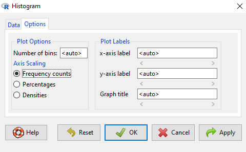
Histogram
Rcmdr: Graphs → Histogram
Select the variable, then select Options to change settings
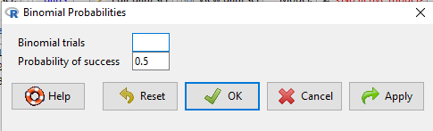
Binomial probability
Rcmdr: Distributions → Discrete distributions → Binomial distribution → Binomial probabilities
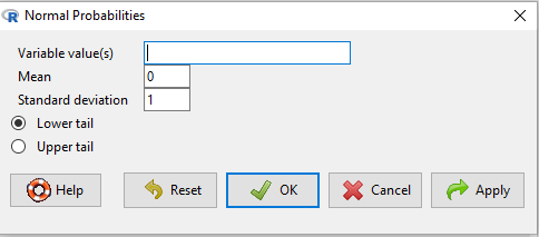
Z-score (normal) problems
Rcmdr: Distributions → Continuous distributions → Normal distribution → Normal Probabilities
Read table of data
darts <- read.table(header=TRUE, sep="\t", text=" ")
Select and copy data including header row and paste between the " " of text = " "
Alternatively, copy and paste data from the table to a spreadsheet file, then import data from the saved spreadsheet file (Rcmdr: Data → Import data → from Excel file…)
Note — the above suggestions are just two possible ways to get the data into R. This very subject was extensively covered in Part 07. Working with your own data. It doesn’t matter how you get the data into R — just that you do! So, try different ways, but settle on what works best for you. Me? I like to work from spreadsheet files, so I copy/paste to spreadsheet, then load into R. However, web scraping is pretty slick, so do invest some time by looking at Part 07. Working with your own data.
Darts data from Fall 2021. Distance was inches from center
| Student | Dart | Distance |
| aar | 1 | 4.72 |
| aas | 1 | 20.87 |
| aat | 1 | 5.51 |
| aau | 1 | 15.75 |
| aav | 1 | 0.79 |
| aar | 2 | 14.96 |
| aas | 2 | 5.12 |
| aat | 2 | 7.09 |
| aau | 2 | 3.54 |
| aav | 2 | 1.57 |
| aar | 3 | 5.51 |
| aas | 3 | 7.48 |
| aat | 3 | 17.72 |
| aau | 3 | 3.54 |
| aav | 3 | 3.54 |
| aaw | 1 | 1.50 |
| aax | 1 | NA |
| aay | 1 | 1.50 |
| aaz | 1 | 1.00 |
| aaw | 2 | 6.50 |
| aax | 2 | NA |
| aay | 2 | 2.40 |
| aaz | 2 | 1.20 |
| aaw | 3 | 8.50 |
| aax | 3 | NA |
| aay | 3 | 11.40 |
| aaz | 3 | 2.00 |
| aaw | 1 | 5.60 |
| aax | 1 | NA |
| aay | 1 | 5.70 |
| aaz | 1 | 1.20 |
| aaw | 2 | 5.00 |
| aax | 2 | NA |
| aay | 2 | 3.50 |
| aaz | 2 | 0.90 |
| aaw | 3 | 2.50 |
| aax | 3 | 11.00 |
| aay | 3 | 2.60 |
| aaz | 3 | 2.20 |
| aaw | 1 | 1.50 |
| aax | 1 | 3.50 |
| aay | 1 | 2.40 |
| aaz | 1 | 2.50 |
| aaw | 2 | 1.50 |
| aax | 2 | 3.50 |
| aay | 2 | NA |
| aaz | 2 | 2.70 |
| aaw | 3 | NA |
| aax | 3 | 5.50 |
| aay | 3 | 6.20 |
| aaz | 3 | 9.50 |
| aba | 1 | 1.28 |
| aba | 2 | 0.98 |
| aba | 3 | 4.23 |
| abb | 1 | NA |
| abb | 2 | NA |
| abb | 3 | NA |
| abc | 1 | 3.44 |
| abc | 2 | 4.41 |
| abc | 3 | NA |
| abd | 1 | 3.74 |
| abd | 2 | 3.62 |
| abd | 3 | NA |