Help with imageJ
On this page I introduce you to imageJ (Schneider et al., 2012) and show, after brief introduction to installing the software or accessing via browser, how to count objects, how to get simple measures of length — straight line and segmented line — and area from a digital image, and even how to extract data from published graphs.
What’s on this page
- Background
- Install imageJ to your computer
- Run imageJ in your browser
- A note about popup menus in browser version of imageJ may hide important functions
- Standard operating procedures
- References
1. Background
From time to time we need to extract data from images. Today, we mostly work from digital images, but the principles date back to photography (e.g., Knaysi 1945; Spurr and Brown 1946). For example, you may need to measure the length of a shell. In general, if a known unit of measure is included in the image, then a calibration can be obtained between number of pixels and units of measurement (mm, cm, etc.). Lengths on uncalibrated images are recorded as number of pixels.
This post is not about how to acquire good quality images suitable for “science,” but instead briefly introduces you to free software that can be used to extract data from images with imageJ. imageJ is wildly used in biology (more than 2000 citations in PUBMED, 20 September 2023). For use of R package digitize, go to Help with R package digitize.
Working with digital images requires image processing software. Some of you have already been introduced to Nikon NX Studio for microscopy (free with registration to download NS Studio). Non-commercial versions also exist, for example, ImageJ. ImageJ is open-source and free to use. Plug-ins have been written by many users to extend the function of ImageJ — I therefore prefer to download and install Fiji (which stands for Fiji is just ImageJ) because Fiji comes with many useful plugins already installed and added to the basic ImageJ program.
ImageJ has been around a number of years, so it has many users who have graciously written programs to extend imageJ capabilities (available as plugins or macros), or provided “how to” tutorials, or both. These can be readily found via Google search. In addition, beginners may wish to work from a book, see Broeke et al (2015).
You can choose to run imageJ in your browser, or install to your computer. Both work although you may find that an installed imageJ on your computer will behave better than the browser version.
2. Install imageJ to your computer
Downloading ImageJ or Fiji for your computer. Decide which software you want
ImageJ (and therefore Fiji) is written in Java, and so can be run on any operating system (e.g., macOS or Windows 11) provided a current “Java run time environment” or “JRE” is installed. If you don’t know what this means, then you can either check to see if your computer has a JRE installed, or try to install and run ImageJ without the included JRE (it’s a smaller download) — if ImageJ won’t run, you’ll need the JRE. The instructions are the same for Fiji.
Note. See IBM What is the Java runtime environment?
3. Run imageJ in your browser
Recently, the good folks who support imageJ have made a version that can be run in your browser, which means you don’t have to install the software onto your computer. For occasional use, the browser version is the way to go. If you analyze images often, install imageJ to your computer. You may access the browser version directly at https://ij.imjoy.io/, or from links at imageJ website.
A note about popup menus in browser version of imageJ may hide important functions
The principles described on this page are the same whether you use imageJ online (in your browser) or installed to your computer. However, I have noticed the popup windows in the browser version may hide some of the functions. For example, to measure lengths we need to convert from number of pixels to units of inches or centimeters. We do this by including a size marker on the image, then call up the Set Scale menu in imageJ (Fig. 1). See Step 3 under Measuring lengths or areas from an image, below.
When you set the scale, the popup window hides “OK” button (Fig. 1), which you need to click to save the settings.
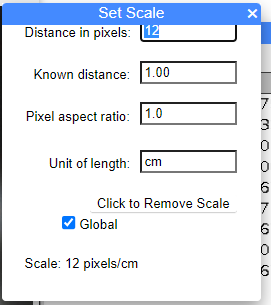
Figure 1. Screenshot of browser version imageJ, note “OK” button is no visible.
To solve this, hover your mouse over the lower right corner to bring up a double white arrow (Fig. 2)
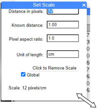
Figure 2. Screenshot of Set Scale menu, browser version of imageJ. Hover mouse over lower left corner and double arrow will show. Hold left-click and drag down to reveal full menu (Fig. 3). Note I added the double arrow and enlarged it for emphasis.
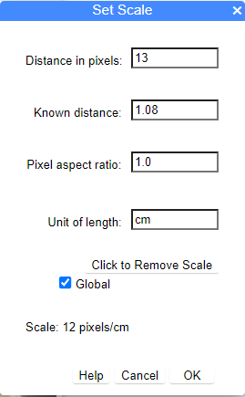
Figure 3. Screenshot of Set Scale, browser version, which shows full menu.
In order to save settings, you need to click OK after making changes.
Standard operating procedures
1. Counting colonies (particles) or other objects
ImageJ makes it easy to count objects from an image. This can be accomplished manually (A. Manual object count) or automatically (B. Automatic counting) if more than a few images are to be analyzed.
A. Manual object count
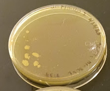
Figure 4. Petri dish with visible yeast colonies
Step 1. Load the image: File → Open
Step 2. Select “Multi-point” picker (red arrow points to menu item, Fig. 5)
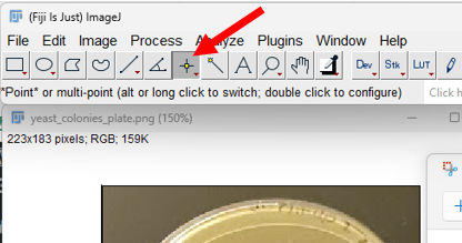
Figure 5. Screenshot imageJ (FIJI) with “Point” menu item visible (red arrow)
Step 3. Click on the down arrow at lower right portion of “Point” menu item. Select Multi-point Tool
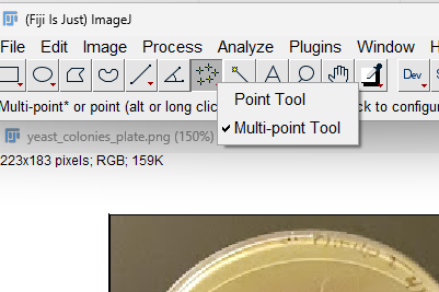
Figure 6. Screenshot imageJ (FIJI) after down-arrow selected, choose “Multi-point tool” from menu
Step 4. Click on colonies or other objects for counting. ImageJ keeps a running tally (the blue plus indicates the pointer is hovering over the next item, before selecting. Yellow dots with numbers — 1, 2, 3, … — are recorded on the image (Fig. 7).
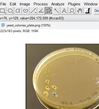
Figure 7. Screenshot imageJ (FIJI) with five multi-points; blue plus indicates live location of pointer before selection.
Step 5. To view the counts (and locations) click imageJ: Analyze → Measure, or Ctrl + M (Command + M) to bring up the Results window (Fig. 8)
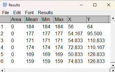
Figure 8. Screenshot imageJ (FIJI) Results window. The first column tracks object counts. Mean, Min, and Max refers to RGB pixels selected; X and Y refers to location of object in the X-Y coordinate system.
Optional. Change measurements displayed in Results. Select Analyze → Set measurements … (Fig. 9).
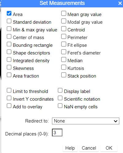
Figure 9. ImageJ screenshot Set Measurements options
B. Automatic counting
If you have lots of plates to count, or the objects are less defined than obvious spots on the image (e.g., counting black spots on a ripe banana), then an automatic procedure applied to multiple images is a better option than simple manual counting.
Step 1. With an image opened (e.g., Figure 4. Petri dish with visible yeast colonies), change to 8-bit. Image → Type → 8-bit
Step 2. Invert image so that colonies are dark on white background: Edit → Invert (Fig. 10).
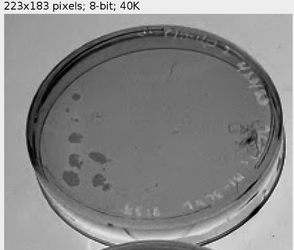
Figure 10. ImageJ screenshot of Figure 4 following 8-bit conversion and inverted image
Step 3. Adjust threshold: Image → Adjust → Threshold. Change to B&W, try different algorithms (e.g., MaxEntropy) to maximize information, minimize background noise. Adjust threshold with slider tool (Fig. 11).
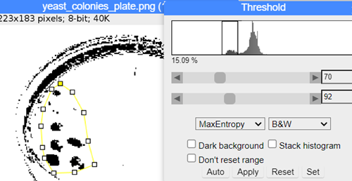
Figure 11. ImageJ screenshot, threshold and ROI
Step 4. Select ROI: Polygon selection tool to encircle colonies on plate (Fig. 11) — note if image was perpendicular to plate, would not need to select ROI
Step 5. Count colonies in ROI: Analyze → Analyze particles… Check Summarize and Exclude on Edges. You may need to adjust the Size from default (0-Infinity) — I found 4-Infinity (just type in “4” in the box, ImageJ will add the range) worked best, i.e., detected the correct number of colonies.
2. Measuring lengths (straight line) or areas from an image or ROI
ImageJ can do lots of things. Here, we introduce only how to record lengths and to calculate areas of interest in numbers of pixels and calibrated units (i.e., unit scale in inches, centimeters, etc.). We’ll use an image of a dart board with three thrown darts. We’ll define two measures: distance in inches between the dart and the center of the board (Length) and the area in squared inches defined by the three darts (Area). An example image is shown in Figure 12.
Note that a more detailed and complete set of instructions for working with the targets is available in SOP_ImageJ_lines. The instructions below are just here to demonstrate basic imageJ features.
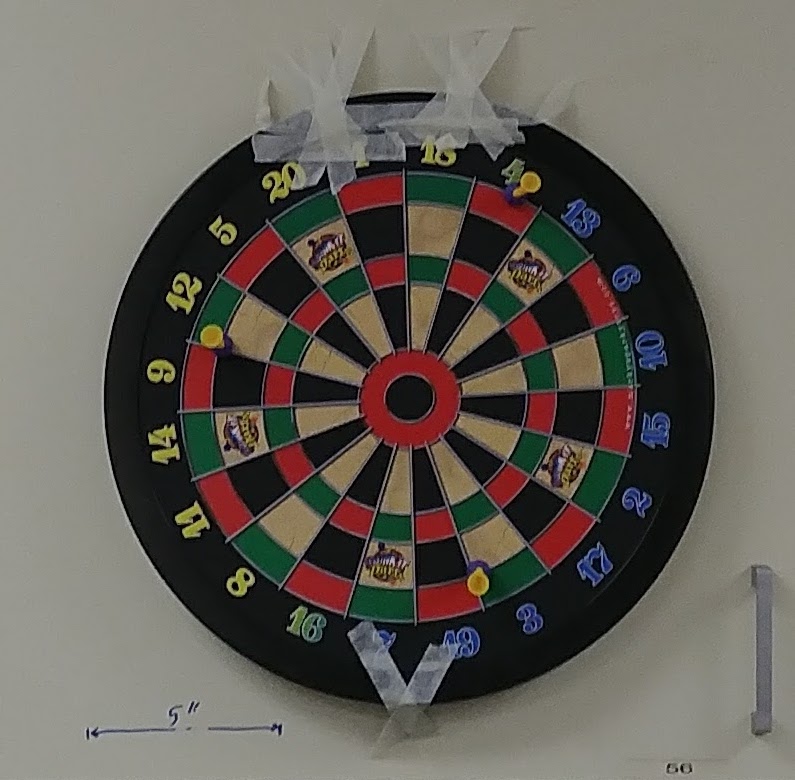
Figure 12. Dartboard inelegantly taped to a metal cabinet door. Note the five inch scale bar at lower left. Alternatively, the diameter of the dartboard was 16 inches.
Step 1. Start ImageJ (or Fiji). Screenshot of Fiji running on a macOS computer is shown in Figure 13.
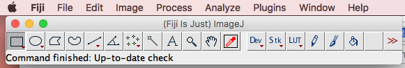
Figure 13. Fiji running on macOS High Sierra
Step 2. Load the image file into ImageJ. File → Open
Step 3. Set the scale to relate pixel count to distance in inches.
- Click on the Line segment tool (Figure 14, red arrow points to the tool); left-click and hold on the down arrow to bring up line tool options
- Straight line: draw a line between two points
- Segmented line: trace an object from one point to another
- Point to the spot/line on the image with known length (e.g., the 5 inch line or the width of the dart board — in this example, the diameter of the board will be the target).
- Click and drag the line across the entire length of the known distance (Figure 15).
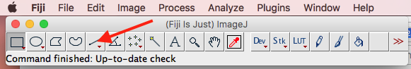
Figure 14. Fiji line tool shown (red arrow). Press and hold the red down arrow to bring up menu (see Fig. 15).

Figure 15. Select straight line to draw line between two points or Segmented Line to incrementally trace a length.
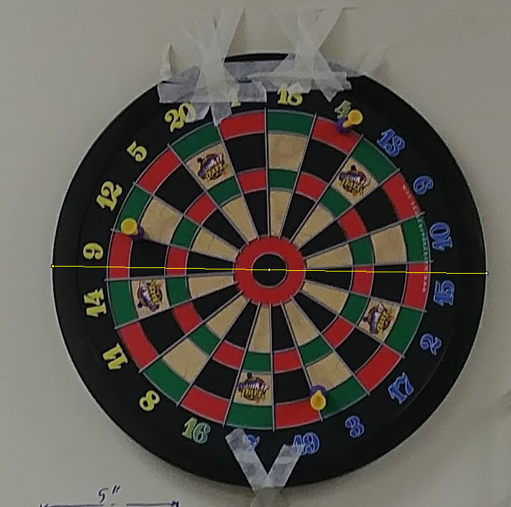
Figure 16. Line drawn to known distance on image, the diameter of the dartboard (16 inches).
Next, select Analyze → Set Scale from the Fiji menu and enter the known distance and set the scale to global (Figure 17).
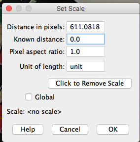
Before setting the scale information |
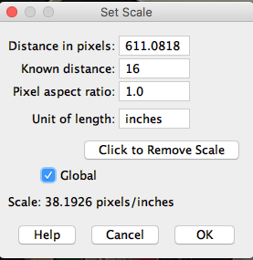
After setting the scale information |
Figure 17. Left, the popup menu with default entries; at right, after the parameters have been entered.
At the end of step 3 you have calibrated number of pixels to number of inches and set the scale for all subsequent measures (global).
Step 4. Return to the image and with the line segment tool selected, draw a line between a dart and the board center (Figure 18).
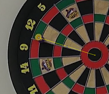
Figure 18. Length of distance between dart and center of board.
Step 5. From the menu, select Analyze → Measure. Default measures will be made by ImageJ and show in the Results window (Figure 19). The distance between the dart location and the center of the board is 5.4 inches.
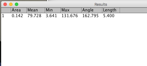
Figure 19. Screenshot of results window
Step 6. Repeat step 4 and 5 for each dart. I get 5.984 and 5.284 inches for dart 2 and dart 3, respectively.
Step 7. To get the area as a measure of dart spread, select the polygon tool from the menu (Figure 20, blue arrow).
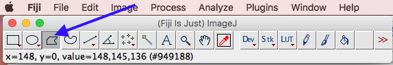
Figure 20. Screenshot of imageJ menu bar, blue arrow points to polygon selection tool.
Click on the first dart to activate the polygon selection tool, then draw towards the second and third darts, ending back on the first dart. Double click to end. A triangle shape should be visible (Figure 21).
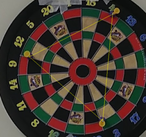
Figure 21. Screenshot of selected polygon region
Step 8. From the menu, select Analyze → Measure. Default measures will be made by ImageJ and show in the Results window (not shown). The area of the polygon is 36.703 inches squared.
3. Use ROI manager to automatically measure area
Will use ROI manager to calculate leaf area of three leaves (Fig. 22). Note that unit scale included with image.
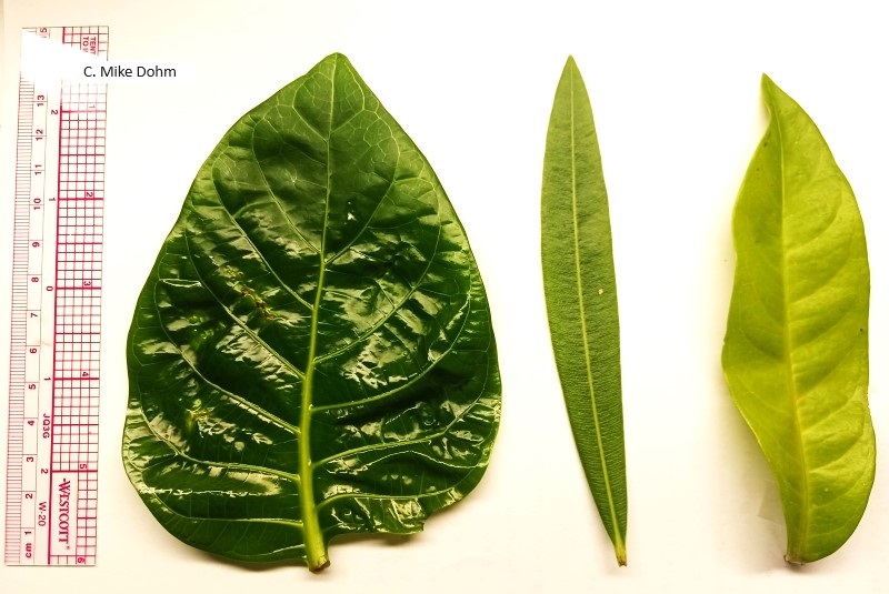
Figure 22. Three leaves with unit scale
Step 1. Load the image, File → Open
Step 2. Adjust image type to 8-bit
Step 3. Apply threshold (Fig. 23)
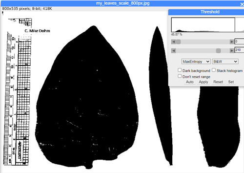
Figure 23. ImageJ screenshot, threshold applied
Step 4. Set scale — see Steps 3 & 4 from above 2. Measuring lengths (straight line) or areas from an image or ROI
Step 5. Analyze → Tools → ROI Manager
Step 6. Select Wand (tracing) tool from the menu bar.
Step 7. With Wand selection tool active, click on the first leaf. Note the leaf edges should automatically be encircled (Fig. 24).
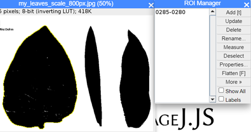
Figure 24. ImageJ screenshot, encircled ROI visible
Step 8. With the first leaf selected, in ROI Manager, select Add [t] (Fig. 24).
Step 9. Repeat Step 7 & 8 for each object (leaf). Three objects should be added to the ROI Manager.
Step 10. In ROI Manager menu, select Measure. Results window will pop up (Fig. 25), displaying measures selected from Analyze → Set Measurements … (see Step 5 & Optional in 1. Counting colonies (particles) or other objects).
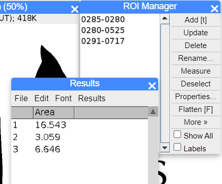
Figure 25. ImageJ screenshot ROI area results
4. Retrieve data from figures in published papers
The following instructions assume you are working with a local installation of imageJ. There is also an R package called digitize that will do the same thing (Help with R package digitize).
Download Figure_Calibration plugin file (Figure_Calibration.class) to the imageJ plugin folder, then restart imageJ. Load the image, then draw a rectangle to define a region in a graph (Figure 14).
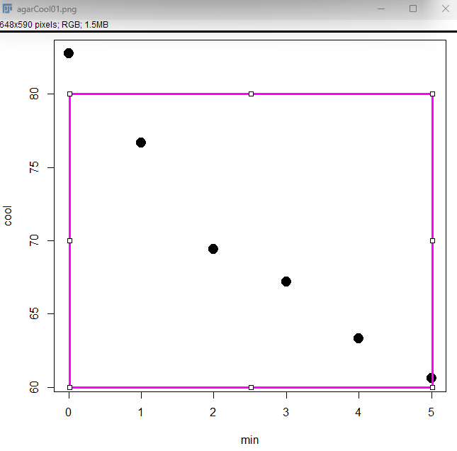
Figure 14. Define region with Rectangle selection tool.
Note: The default selection color is yellow with a thin line (width = 1). To change, Edit → Selection → Properties. Rectangle selection Figure 13 properties : stroke color = magenta, width = 3.

Figure 15. Select Figure Calibration plugin
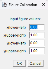
Figure 16. Default popup menu, Figure Calibration
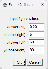
Figure 17. Enter values for X-axis (0, 5) and for Y-axis (60, 80)
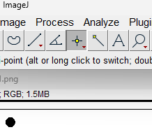
Figure 18. Choose the Point tool

Figure 19. Click on a point, then from menu select Analyze → Measure. View Results.
7. References
Broeke, J., Mateos Perez, J. M., & Pascau, J. (2015). Image Processing with ImageJ, 2nd Edition.
Knaysi, G. (1945). On the microscopic methods of measuring the dimensions of the bacterial cell. Journal of Bacteriology, 49(4), 375-381.
Schneider, C. A., Rasband, W. S., & Eliceiri, K. W. (2012). NIH Image to ImageJ: 25 years of image analysis. Nature methods, 9(7), 671-675.
Spurr, S. H., & Brown, C. T. (1946). Tree height measurements from aerial photographs. Journal of Forestry, 44(10), 716-721.