Part 03. Explore use of R
Instructions on this page are general to use of R and apply to R used on local computer or to users of R in Google CoLab.
Learning objectives
- Apply R as a calculator and evaluator of arithmetic and expressions.
- Manipulate logical, relational, and date/time data.
- Create simple plots and leverage R’s built-in functionality for linear algebra and calculus operations.
What’s on this page?
- Explore use of R as a calculator
- Work with time and date values
- Explore use of logical and relational operators in R
- Make a simple plot with
plot() - Have R clean up a URL
- R can do Linear Algebra
- Evaluate an expression
- R can do Calculus
- Work with the script window
- Quiz
What to do
Complete the exercises on this page
- Explore use of R as a calculator
- Explore use of logical and relational operators in R
- Practice use of R to evaluate expressions
- R can do Calculus
- R can do Linear Algebra
How to do it
For these exercises, you may work
- within the Rcmdr script window
- at the command line and R prompt
- from a script document and the R GUI app
- RStudio
Choose one way. The quickest way is to just work within R.
Let’s begin.
Before you start
A reminder, always set your working directory in R first (see Part 02. Getting started with R and Rcmdr), before starting to do your analyses. Makes life a lot easier.
1. Explore use of R as a calculator
Question 1. Collectively, what are the “+”, “-“, “*”, “/” symbols called? (You don’t need R to answer this question).
A) arithmetic operators
B) functional operators
C) logical operators
D) relational operators
E) All of the above
Question 2. At the prompt (>), use R to calculate answers to the following simple equations, one at a time (don’t type the prompt!). Note that in the R script, the prompt is not visible.
4 + 4
4 - 4
4 * 4
4 / 4
Repeat calculations on the simple equations, but this time, assign each answer to an object, then print the object (“Everything in R is an object”). R uses “=” and “<-” to assign. It’s recommended that you use “<-“.
- For example
firstEq <- 4 + 4
Repeat for the other calculations, assigning each a unique object name. What do you see when you hit enter?
Question 3. When you submit the above equation/command, what shows up at the R prompt?
- To print the object, just type the object name at the R prompt
firstEq
- to print the object automatically, add a semicolon to the end of the statement and repeat the name of the object. For example, edit the first command as follows
firstEq <- 4 + 4; firstEq
R can work with dates and times, and you can do calculations on these types as well. For example, the command to get today’s date is
Sys.Date()
To do: Observe and interpret the output from each entry.
2. Work with time and date values
Question 4. Create an object like firstEq called today and assign a value to the object returned by Sys.Date(). Print the object.
How many days are there until your graduation date? Create a date object for the graduation date, formatted like the next example
#replace the date with your expected graduation date.
nextGrad <- c("2022-5-8")
where c is short for combine.
Now, you have to tell R to treat this object as a date, so use the next command
nextGrad <- as.Date(nextGrad)
And finally, subtract the Sys.Date (or today, the stored object!) from the nextGrad object
nextGrad - Sys.Date()
Question 5. What day did I first publish this page? What date did I last modify this page? Hint: use your browser’s “View page source” and search for datePublished and dateModified, respectively.
And if you want the number of weeks and not days? Use difftime, like in the next example.
difftime(nextGrad, Sys.Date(), units = "weeks")
Question 6. What date format was used for this page? Hint: right click this page in your browser, then select View page source (Chrome, Edge) or Show page source (Safari). Search for “time” or “date.”
A) %m/%d/%y
B) %m-%d-%y
C) %y/%m/%d
D) %y-%m-%d
Question 7. Try the difftime function, but calculate for a difference of months, not weeks.
Note 1: There is much more to do with times and dates. This was just a starter. For more information about working with times and dates in R, see https://www.r-bloggers.com/using-dates-and-times-in-r/ .
Difference between any two dates, how to work with date formats
date1 <- as.Date("12/4/20",format="%m/%d/%Y"); date1
date2 <- as.Date("3/4/21",format="%m/%d/%Y"); date2
difftime(date2,date1,units="days")
3. Explore use of logical and relational operators in R
Boolean algebra is a kind of algebra to describe logical relations as opposed to numerical relations. Instead of simple algebra where the values of the variables are numbers, and the operations are addition, multiplication, etc., Boolean algebra operations are the conjunction (AND), the disjunction (OR), and the negation (NOT). Boolean operators return values of TRUE or FALSE. Because R is a programming language it has full command of Boolean operators.
Question 8. Logical operators in R include X|Y (X OR Y), X&Y (X AND Y), and all of the relational operators. Relational and logical operators are useful programming operators for making comparisons or for filtering data based on a test criteria. The next examples show how to work with relational operators.
Note 2: The hashtag, #, is used in R to write comments in your code. R won’t do anything with text that follows a hashtag.
#Is 4 less than 5?
4 < 5
Question 9. Use R to test whether or not 4 + 5 is exactly equal to 5 + 2*2 (hint: use ==).
Question 10. Make a sequence of numbers between 1 and 5 and assign to object “seqx”.
Example
#create a sequence from 1 to 20, assign to object x
x <- c(1:20)
What is the R output for x? For seqx?
Question 11. If we want to subset numbers less than or equal to 4 from x, our vector of a sequence of numbers from 1 to 20, we might select
#subset from x all numbers less than or equal to 4 and assign to a new object
y <- x[(x<=4)]
Note 3: In R, parentheses like “(” and “)” are for functions and setting order of operations of calculations. Square brackets “[” and “]”are for indicating position in vectors. R also recognizes and uses curly braces “{” and “}” for several key purposes, including to group multiple expressions into a single block of code like a for loop in a function.
Repeat, but this time select subset for all numbers greater than 15. Assign this to suby
What is the R output for y? For suby?
Question 12. Using relational and logical operators, assign to object z all numbers from x that are less than or equal to 4 OR greater than 12.
We created a series of numbers by assigning the sequence between 1 and 20 using the colon. A more generic function is seq() and it is demonstrated here. The command takes three inputs: starting number, ending number, and the size to increment. Before we wrote
x <- c(1:20)
with seq() this would be written as
x <- seq(1,20,by=1)
Note 4: this overwrites our previous x. R will do this without warning you, so be aware!
etc.
Note 4: this overwrites our previous x. R will do this without warning you, so be aware!
To do: Print x; what was the R output for x?
Repeat, but change by=1 to by=4 and report the R output
Question 13. Create a new object y with values 11 through 52, incremented by 2. What is the value of the 13th element in the object y?
Answer. Type at the R prompt
y <- seq(11,52, by=2)
y[13]
And R output is…?
Click here for the answers: Answers: Explore
4. Make a simple plot with plot()
R has a whole bunch of graphics capabilities, particularly if you add packages like ggplot2. However, the base installation has a number of graphics commands, and we’ll start there with plot(). Consider data on rate of cooling of agar. Making agar plates is a routine task in biology lab; melting temperature of agar is about 85 °C while ideal pouring temperature is between 60 and 70 °C.
| Min | Trial01 | Trial02 | Trial03 | Trial04 |
|---|---|---|---|---|
| 0 | 82.8 | 88.7 | 83.2 | 86.2 |
| 1 | 76.7 | 78.5 | 77.6 | |
| 2 | 69.4 | 74.3 | 72.5 | 74.3 |
| 3 | 67.2 | 71.4 | 70.7 | 68.9 |
| 4 | 63.3 | 67.6 | 68.5 | 61.5 |
| 5 | 60.6 | 65.5 | 65.8 | 57.7 |
| 6 | 63.9 | 62.3 | 54 | |
| 7 | 59.9 | 61.5 | 53.4 | |
| 8 | 56.7 | 58.6 | 50.6 | |
| 9 | 56.3 | 48.2 | ||
| 10 | 55 | 55.4 | 46.7 |
We need to get the data into R, which is the subject of Part 07. Working with your own data.
Note 5: If it was me, I would just copy from the table, paste it into a spreadsheet, then import to R from the spreadsheet with commands available in rio package; columns would be tab-delimited. It’s also a good candidate for web scraping, see code to do just this: Web scraping from a static webpage (rvest package) at Part 07 – Working with your own data
For now, I’ll give you the code and data — let’s just enter directly
myCool <- read.table(header=T, sep=",", na.strings="NA", text="
Min,Trial01,Trial02,Trial03,Trial04
0,82.8,88.7,83.2,86.2
1,76.7,78.5,77.6,NA
2,69.4,74.3,72.5,74.3
3,67.2,71.4,70.7,68.9
4,63.3,67.6,68.5,61.5
5,60.6,65.5,65.8,57.7
6,NA,63.9,62.3,54
7,NA,59.9,61.5,53.4
8,NA,56.7,58.6,50.6
9,NA,56.3,NA,48.2
10,NA,55,55.4,46.7")

# Check the data entry
head(myCool)

# Make scatterplot with one trial, e.g., Trial02
plot(myCool$Min, myCool$Trial02, pch=19, cex=1.5, xlab="minutes", ylab="degrees Celsius", main="Agar cooling curve")

# Make a smoothed line with lowess
lines(lowess(myCool$Min, myCool$Trial02), col="red")

Figure 1. Agar heated in microwave, cooling data
# Make plot with all trials
matplot(myCool[,2:5], type="p", pch=19, cex=1.5, lty=1, lwd=2, col=c("blue", "yellow", "red", "green"), xlab="Minutes", ylab="deg C", main="Agar cooling curve")
legend("right", c(myCool[,2:5]), lty=1, col = c("blue", "yellow", "red", "green"), box.lwd = 0)
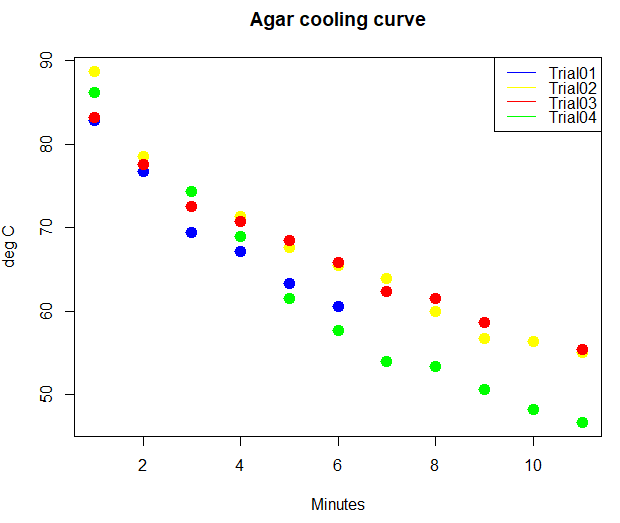
Figure 2. Agar heated in microwave, four trials cooling data
Brief remarks about the code. na.strings="NA" informs R that missing values are denoted as Not Available. (See Mike’s Biostatistics Book for discussion about missing values in Chapter 5 – Experimental design.)
Instructions like type = "p", pch, cex, lty, lwd, and col are plot parameters. I can tell you what each does (or you can look it up, type \?par at the R prompt to bring up the help page), explore the settings by changing and making new plots. For example, change type = "l" and redo the plot; change lty = 2, remake the plot, etc.
Note 6: Yes, that’s some messy data in Figure 2! Without getting defensive, records were made by different people using different — and uncalibrated — IR thermometers. OK, that was a little defensive.
5. Have R clean up a URL
I often ask students to send me links in support of their work. Cookies are commonly attached to the url to keep track. A copy/paste on the url generates a ridiculously long, and error prone address. For example, following a link, the url to Mike’s Biostatistics Book might look like
The url we want is https://biostatistics.letgen.org — Everything after the “?” is the tracking cookie. We use the function str_extract() from the R package stringr.
library(stringr)
my_string <- "https://biostatistics.letgen.org/?_gl=1%2A194hw8n%2A_ga%2AMTAzNjg1OTE5MS4xNzY1OTI3MTMz%2A_ga_P3JKKCEJPM%2AczE3Njg5Mzk2NzEkbzIwJGcwJHQxNzY4OTM5NjcxJGo2MCRsMCRoMA.."
str_extract(my_string, "^[^?]+")
returns the URL we want.
6. R can do Linear Algebra
Linear algebra is a branch of mathematics concerned with linear equations with the components represented by vectors and matrixes (Britannica). Vectors are lists of numbers, matrixes are arrays of numbers with dimensions determined by number of rows and columns. Vectors can be thought of as a matrix with one column and multiple rows. Vectors have both direction and magnitude, and are often expressed by coordinates: in 2D, each ith point (element, e.g., i = 1 to 10) in the vector is represented by an X value and a Y value and would be represented as (
![\[x_{i}, y_{i}\]](https://mikeworkbook.letgen.org/wp-content/ql-cache/quicklatex.com-9a82d8ed235c52775dd0c34af80c494b_l3.png "Rendered by QuickLaTeX.com")
); in 3D, each ith point (element, e.g., i = 1 to 10) in the vector is represented by an X value, a Y-value, and a Z value and would be represented as (
![\[x_{i}, y_{i}, z_{i}\]](https://mikeworkbook.letgen.org/wp-content/ql-cache/quicklatex.com-e19faa63a919915c35454a49f9396852_l3.png "Rendered by QuickLaTeX.com")
), and so on. Like calculus, linear algebra is an important tool in systems biology.
Base R can do linear algebra.
7. Evaluate an expression
R can be used to explore or “evaluate” algebraic expressions. For example, it has long been known in biology that organisms grow “allometrically.” That is, the relative change in proportions of organism traits in relation to total body size follows the allometric equation

where y is any biological variable, Mass refers to body weight of the organism, and b is the scaling exponent. Allometric equation is an example of a power equation. We’ll revisit allometric equations when we discuss linear and nonlinear models (Chapter 17, 18). Note that if the scaling component is equal to one, then rate of change is directly proportional to increase in mass, i.e., isometric growth. If the scaling component is less than one, then the trait changes at a rate less than proportionality. And lastly, if the scaling component is greater than one, then allometric change is out of proportionality. Famous allometric equations include rate of metabolism or Kleiber’s law

where Metabolic rate is kcal per day and Mass is in kilograms.
We can use R to explore the equation. First, use expression() to assign the equation.
kleiber <- expression(a*Mass^b)
where kleiber holds the object.
Next, set up your constants and the Mass variable with values.
a = 67
b = 0.75
Mass <- c(0.1, 1, 10, 100)
Use eval() to evaluate the model with the specified values. Assign results to an object.
y <- eval(kleiber); y
Question 14. Carry out the evaluation of Kleiber’s equation for the values given. What does the plot of Metabolic rate on Mass look like?
Hint: the R function to make a plot is simply
plot(x,y)
8. R can do Calculus
The base R package includes routines to get derivatives from equations. As you hopefully recall from your calculus, the first derivative gives you the rate of change or slope of the tangent to any curve; it tells us whether the function increases or decreases. The second derivative tells us instantaneous rate of change of the first derivative.
The function call to get the first derivative is simply
D(expression, "x")
and the second derivative would be obtained by
D(D(expression, "x"), "x")
where “x” is used to specify that derivation has to be carried out with respect to x.
Question 15. Get the first and second derivatives of Kleiber’s equation with respect to Mass.
Question 16. Use the first derivative to evaluate the increase of metabolic rate when body mass increases from 10 to 11 kg.
Question 17. Use the second derivative to evaluate the change of sloped of Kleiber’s equation when body mass increases from 10 to 11 kg.
9. Work with the script window
While you can enter instructions one line at a time, pretty soon this isn’t a viable option. For example, when you create functions it is often best to write the functions over multiple lines (functions instructions are enclosed between {}). Thus, R comes with the ability to handle scripts. Scripts can contain hundreds of lines of commands. You then highlight the lines of code you want to run and submit them at once. The RGUI allows you to create script documents: File → New document, and you submit code to run by placing the cursor on the code line and entering keyboard combination Ctrl + Enter (on macOS, replace with Cmd + return keys). But for us, it’s easier to take advantage of the Rcmdr script window.
Thus, if you have not already done so, start R Commander (again, type at the R prompt
library(Rcmdr)
and repeat the examples/questions above, but this time using the script window.
10. Page quiz.
Explore R
Seven questions from this page