Homework 6: Chi-square problems
Homework objectives
- Differentiate and chose between goodness of fit and contingency table chi-square analysis
- Practice use of R to conduct statistical tests.
- Practice reading and extracting R output from statistical commands.
- Evaluate error rates (Type I, Type II) and critical value, p-value.
Homework 6 expectations
BI-311 students: For homework reports, report only your answers for the even numbered questions. There’s also a BONUS, with six questions for you to consider. Read through the entire homework before starting to answer a question — all questions are intended to help you achieve the learning outcomes for the chapter. You are expected to have read the chapter and to have completed preceding homework. Answers are provided to odd numbered problems — turn in your work for even numbered problems.
How to work this homework
You may work together, but each of your must turn in your own report. Don’t “plagiarize” from each other. Do include in your report who you worked with.
What to turn in: A pdf file containing relevant R code, statistical results — edited to support your answers to the questions, and your answer to the questions (even numbered only). Use of RMarkdown recommended — because it is a simple way to include graphs generated; however copy/paste into a word document is also acceptable.
Notes. By relevant we mean provide just the R code and results from R functions necessary to support your answers to the questions. For example, do not include
- the entire data set when head(dataset) will do
- screenshots of R output!! R output is text — copy/paste
- all statistical output from an R function.
See Part09: Making a report for an example homework file.
Submit your work to CANVAS. Obey proper file naming formats.
Resources for this homework
Chapter 9. Mike’s Biostatistics Book
Mike’s Workbook for Biostatistics: A quick look at R and R Commander, Part01 – Part10 and previous homework pages presented in this workbook.
Additional R commands and or code provided below.
Questions
1. Testing for homogeneity of Mendel’s data on seed shape in five F2 plants. (Hint: first get the test for all 5 plants combined, then try separately for each plant. Try the 3:1 ratio for the null hypothesis.)
| Plant | Observed Round seeds |
Expected Round seeds | Observed Wrinkled seeds | Expected Wrinkled seeds | χ2 | p-value |
| 1 | 45 | 12 | ||||
| 2 | 27 | 8 | ||||
| 3 | 24 | 7 | ||||
| 4 | 19 | 10 | ||||
| 5 | 32 | 11 | ||||
| Total | 147 | 48 |
- Is this a “goodness of fit” or a “contingency table type” of problem?
- Should you apply the Yate’s correction?
- Write out the null and alternative hypotheses, then test the null hypotheses.
- Complete the table.
2. How many experimental units in Mendel’s experiments on seed shape?
-
- One
- Five
- Forty-eight
- One hundred forty-seven
- One hundred ninety-five
3. At what level is there replication in Mendel’s experiment
-
- Parental plants
- F1 plants
- F2 plants
- None of the above
4. One hundred thirteen (113) F2 tomato seeds were planted in hydroponics setup, grown for two weeks, then scored for leaf color. F2 of tomato progeny from F1 of cross between YY and yy plants, y is lethal in homozygous recessive, plants don’t live much past two weeks. In contrast to complete dominance, the F1 leaf morph is a blend of the two parents, thus exhibiting incomplete dominance. Leaf color of YY is green, the heterozygote Yy are green-yellow, and the yy homozygote are yellow. Fifteen seeds failed to germinate.
| Phenotypes | Observed counts | Expected |
| Green | 30 | |
| Green-Yellow | 49 | |
| Yellow | 19 |
- Is this a “goodness of fit” or a “contingency table type” of problem?
- Write out the null and alternative hypotheses, then test the null hypothesis.
- What if all 15 seeds that failed to germinate were of the yy genotype? Repeat your analysis and compare the results.
5. A dihybrid cross between tall, potato-leaf tomatoes and dwarf, cut-leaf tomatoes. Assume tall dominant over dwarf, cut leaf dominant over potato-leaf. Write out the null and alternative hypotheses, then test the null hypothesis.
| Phenotypes | Observed Counts | Expected |
| Tall, cut-leaf | 926 | |
| Tall, potato-leaf | 288 | |
| Dwarf, cut-leaf | 293 | |
| Dwarf, potato-leaf | 104 |
data cited by Sokal and Rohlf 1995, Biometry, 3rd ed.
- Is this a “goodness of fit” or a “contingency table type” of problem?
- Write out the null and alternative hypotheses, then test the null hypothesis.
6. An early study on the effectiveness of a potential treatment of AIDS (progression defined as a substantial decrease of CD4+ cells). Write out the null and alternative hypotheses, then test the null hypothesis.
|
AZT Treatment
|
||
| Disease Progressed | No Progression | |
| AZT |
76
|
399
|
| Placebo |
129
|
332
|
| NEJM 329:297-303, 1993 | ||
- Is this a “goodness of fit” or a “contingency table type” of problem?
- Should you apply the Yate’s correction?
- Write out the null and alternative hypotheses, then test the null hypothesis.
7. The association between early diabetic nephropathy on mortality and type 2 diabetes in a sample of men 50-75 years (diabetes diagnosed by age 45). At the start of the study, each subject was characterized as having normal or abnormally low levels of albumin excretion. The subjects were followed for 10 years. Write out the null and alternative hypotheses, then test the null hypothesis.
|
Albumin excretion group
|
||
| low | normal | |
| Died |
55
|
59
|
| Survived |
73
|
17
|
| NEJM 310:356-360, 1984 | ||
- Is this a “goodness of fit” or a “contingency table type” of problem?
- Write out the null and alternative hypotheses, then test the null hypothesis.
- Test the null hypothesis; report the results.
- What can we conclude about the statistical evidence for/against the null hypothesis
8. Vienna Maternity Hospital in Germany had two clinics. From 1840 through 1846, the maternal mortality rate in the first clinic was 98 per 1000 births, while the rate in the second clinic – the midwives clinic – was only 36 per 1000 births. Almost all the maternal deaths were due to puerperal fever. (You may recognize this story — it’s about the hospital that Ignaz Phillip Semmelweis worked; he’s famous for introducing importance of hand washing by health-care workers.)
- Is this a “goodness of fit” or a “contingency table type” of problem?
- Write out the null and alternative hypotheses
- Test the null hypothesis; report the results.
- What can we conclude about the statistical evidence for/against the null hypothesis
9. Bumpus reported differences in body size that correlated with survival (Bumpus 1899), and this report is often taken as an example of Natural Selection (cf. Johnston et al 1972). The study was discussed in Question 5, Chapter 5 of Mike’s Biostatistics Book, and again in Chapter 5.6 of Mike’s Biostatistics Book.
Table 1. Bumpus data set, summarized by sex of birds.
| House sparrows |
Lived | Died |
|---|---|---|
| Female | 21 | 28 |
| Male | 51 | 36 |
- Is this a “goodness of fit” or a “contingency table type” of problem?
- Write out the null and alternative hypotheses
- Test the null hypothesis; report the results.
- What can we conclude about the statistical evidence for/against the null hypothesis.
BONUS
Six additional questions for bonus opportunity.
First, run a simple chi-square test example: Mendel dihybrid cross
peas <- c(315,101,108,32)
# If p equal, then rep(prob,count)
prob <- c(9/16, 3/16, 3/16, 1/16)
# We want to keep track of p values. We use str(ing) command to
# see how the test saves p values we then can extract.
out <- chisq.test(peas,p=prob)
out
str(out)
Second, run chi-square analysis on a new data set. Here’s the class counts of colors for bags of chocolate M&Ms.
# Data set from Fall BI311 and BI216 students
# This is a wide format.
myData <- read.table(header=TRUE, sep=",", text="
bag, Blue, Green, Yellow, Orange, Red, Brown
a, 2, 5, 1, 8, 1, 0
b, 2, 7, 4, 3, 1, 1
c, 2, 3, 1, 5, 2, 1
d, 1, 4, 4, 4, 0, 3
e, 0, 4, 3, 4, 5, 1
f, 2, 5, 0, 2, 0, 4
g, 2, 4, 6, 3, 0, 1
h, 3, 5, 4, 1, 3, 1
i, 3, 3, 4, 2, 1, 3
j, 2, 3, 2, 7, 2, 1
k, 2, 3, 4, 5, 0, 1
l, 1, 5, 3, 4, 1, 2
m, 1, 4, 5, 3, 0, 4
n, 1, 5, 1, 10, 2, 0
o, 3, 1, 3, 6, 1, 2
p, 1, 3, 1, 5, 1, 4
q, 3, 3, 5, 2, 0, 2
r, 3, 7, 1, 3, 0, 2
s, 2, 4, 4, 4, 1, 0
t, 0, 4, 3, 1, 4, 3
u, 3, 6, 1, 3, 0, 3
v, 5, 4, 4, 0, 1, 2
w, 3, 2, 1, 4, 2, 2
x, 0, 6, 3, 3, 1, 2
y, 2, 3, 0, 4, 1, 6
z, 3, 1, 2, 4, 1, 3
aa, 3, 3, 1, 3, 2, 4
ab, 1, 6, 2, 3, 1, 3
ac, 3, 3, 3, 5, 0, 2
ad, 0, 3, 3, 7, 1, 1
ae, 2, 6, 3, 3, 2, 0
af, 2, 5, 2, 3, 0, 2
ag, 3, 1, 3, 6, 0, 3
ah, 4, 2, 2, 3, 3, 1
ai, 3, 5, 3, 3, 1, 1
aj, 1, 3, 5, 5, 1, 0
ak, 0, 2, 4, 2, 2, 5
")
head(myData)
attach(myData)
# Need a matrix to get the counts. Drop bag variable.
counts_matrix <- as.matrix(myData[, -1])
# Or equivalent code
# counts_matrix <- as.matrix(myData[, 2:ncol(myData)])
chisq.test(counts_matrix)
Bonus Question 1. Interpret the test of the null hypothesis.
Bonus Question 2. If instead of combining the bags we ran a chi-square test on each bag, (a) how many total tests (comparisons) would we run and (b) how many tests would we expect to be significant at alpha = 5% by chance alone?
Now, conduct tests on each bag and save the p-values. Include Yates correction.
Bonus Question 3. We didn’t run Yates correction for the collected counts. Why must we apply Yates correction when we conduct tests on each bag?
The R code
numRows <- nrow(counts_matrix)
p_values <- numeric(numRows)
myProb <- rep(1/6, 6)

for (i in 1:numRows) {
     suppressWarnings({
      test_result <- chisq.test(counts_matrix[i, ], p = myProb, correct=TRUE)
       })
      p_values[i] <- test_result$p.value
     }

print(p_values)
sum(p_values < 0.05)
# Expect
numRows*0.05
Bonus Question 4. Compare how many p-values less than 5% to how many we expected by chance.
Bonus Question 5. This example relates to our discussion of multiple comparisons — What is the best explanation for the number of significant tests, random variation or do we need an alternative explanation, eg, cost of dye differences?
Bonus Question 6. Treat this problem as a “meta-analysis.” Test heterogeneity of p-values using Fisher’s method. Do we have evidence to reject the “equa; frequencies” null hypothesis?
R code follows
# Option one, add totals, run single chisq.test -- which we already did!
# Option two, test heterogeneity via fisher's method
# Requires package poolr, install first.
# Introduced fisher's method Ch 12.4
install.packages("poolr")
library(poolr)
my_P <- p_values
fisher(my_P)
Additional R or Rcmdr commands
Chi-square “goodness of fit” (gof) test
chisq.test (c(O1, O2, ... On), correct = FALSE, p =(c(E1, E2, ... En)))
where O1, O2, ... On refer to counts of first group observations, second group observations, and so on up to the nth group. E1, E2, ... En correspond to the expected counts for group 1, group 2, and so on up to the nth group.
Example
I’ll do the first plant from problem 1. You could plug in the numbers, one pair at a time, but here’s a simple way to take advantage of R’s indexing system. I create an object and store the records for each of the five plants. I then call the element by number to retrieve the counts for plant 1 by adding [1] after the name of the object.
round <- c(45, 27, 24, 19, 32)
wrinkled <- c(12, 8, 7, 10, 11)
chisq.test (c(round[1], wrinkled[1]), p =(c(0.75, 0.25)))
and the results were
Chi-squared test for given probabilities

data: c(round[1], wrinkled[1])
X-squared = 0.47368, df = 1, p-value = 0.4913
The 2X2 contingency table analyses
Assuming you have already summarized the data, you can enter the data directly in the Rcmdr contingency table form
Doll and Hill (1950) Example
| Smokers | Non-smokers | |
| Case controls, no lung cancer | 622 | 27 |
| Lung cancer | 647 | 2 |
Statistics > Contingency tables > Enter and analyze two-way table… (Fig. 1)
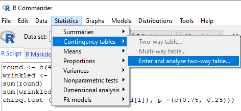
Figure 1. Screenshot, select enter and analyze two-way table Rcmdr menu
Enter your numbers (Fig. 2)
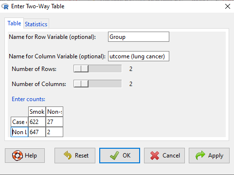
Figure 2. Screenshot with 2×2 data entered
Next, select Statistics tab and select options. Default Hypothesis test is the chi-square option (Fig. 3).
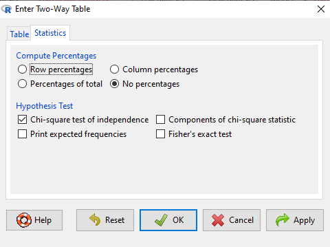
Figure 3. Screenshot Rcmdr 2×2 statistics options.
After completing the 2×2 entry, click OK button. Results were
Pearson's Chi-squared test

data: .Table
X-squared = 22.044, df = 1, p-value = 0.000002664
Note: Rcmdr reports the commands. For our report, we want the answer of the hypothesis test, so the edited version of the complete output is shown above.
2X2 Contingency table: Use RcmdrPlugin.EBM as alternative
If you have not already done so (Chapter 7 we introduced you to this plugin), download and install RcmdrPlugin.EBM (Leucuta et al 2014).
install.packages("RcmdrPlugin.EBM")
Then, from Rcmdr, select Tools > Load Rcmdr plugin(s)… and select RcmdrPlugin.EBM from the list. Close and restart Rcmdr and locate the EBM menu. Select Enter two-way table… and proceed as before. The EBM has additional options. Pay attention to how you set up the tables. For data consistent with Prognosis option, the table should be set up as
| Disease + |
Disease – |
|
| Exposure + | ||
| Exposure – |
References
LEUCUȚA, D. C., CĂLINICI, T., Drugan, T., Istrate, D., & ACHIMAȘ, A. (2014). Graphical User Interface Extension in R Commander for Evidence Based Medicine Indicators. Applied Medical Informatics., 35(3), 11-16.
Loudon, I. (2013). Ignaz Phillip Semmelweis’ studies of death in childbirth. Journal of the Royal Society of Medicine, 106(11), 461-463.
Sokal, R.R. and Rohlf, F.J. (1995) Biometry: The Principles and Practice of Statistics in Biological Research. 3rd Edition, W.H. Freeman and Co., New York.