Answers: Multiple linear regression
Homework 11: Multiple linear regression
Answers to selected number problems
1.
a. Region, Division, State, County all categorical, nominal
names(cancer_reg)

"TARGET_deathRate" (ratio)     "Region" (nominal)           "Division" (nominal)
"State" (nominal)              "County" (nominal)           "medIncome" (ratio)
"popEst2015" (ratio)           "povertyPercent" (ratio)     "studyPerCap" (ratio)
"MedianAge" (ratio)            "AvgHouseholdSize"           "PercentMarried" (ratio)
"BirthRate" (ratio)            "PctHS25_Over" (ratio)       "PctBachDeg25_Over" (ratio)
"PctUnemployed16_Over" (ratio) "PctPrivateCoverage" (ratio) "PctPublicCoverageAlone" (ratio)
"PctWhite" (ratio)             "PctBlack" (ratio)           "PctAsian" (ratio)
"PctOtherRace" (ratio)
b. TARGET_deathRate = dependent variable
all other variables independent variables
c. Therefore, TARGET_deathRate response variable and all other variables potential predictor variables
d. Factors are the nominal variables: Counties nested in States, States nested in Division, Division nested in Region.
3. Note: a full model is not the best model choice. Many of the predictor variables are correlated, hence, the full model violates basic assumptions about model building, i.e., predictor variables are independent.
a. Dependent variable is TARGET_deathRate. Lots of possible simpler models. To illustrate a multiple regression, I selected these ratio variables
Region
AvgHouseholdSize
MedianAge
medIncome
PctPublicCoverageAlone
PctUnemployed16_Over
PctWhite
PercentMarried
povertyPercent
Lots of socioeconomic factors are associated with increased cancer risk and mortality. A couple of highlights from my selection: I predict negative linear association between cancer mortality and percent of population that is White (a well known health disparity).
b. Rcmdr: Statistics → Summaries → Correlation matrix…
This returns a symmetric matrix of correlations (above and below the diagonal are identical). Pearson correlations:
                AvgHouseholdSize MedianAge medIncome PctPublicCoverageAlone PctUnemployed16_Over PctWhite PercentMarried povertyPercent
AvgHouseholdSize          1.0000 -0.0319  0.1121  0.0611  0.1315 -0.1884 -0.1005  0.0743
MedianAge                -0.0319  1.0000 -0.0133 -0.0033  0.0186  0.0350  0.0464 -0.0293
medIncome                 0.1121 -0.0133  1.0000 -0.7198 -0.4531  0.1672  0.3551 -0.7890
PctPublicCoverageAlone    0.0611 -0.0033 -0.7198  1.0000  0.6554 -0.3610 -0.4600  0.7986
PctUnemployed16_Over      0.1315  0.0186 -0.4531  0.6554  1.0000 -0.5018 -0.5515  0.6551
PctWhite                 -0.1884  0.0350  0.1672 -0.3610 -0.5018  1.0000  0.6774 -0.5094
PercentMarried           -0.1005  0.0464  0.3551 -0.4600 -0.5515  0.6774  1.0000 -0.6429
povertyPercent            0.0743 -0.0293 -0.7890  0.7986  0.6551 -0.5094 -0.6429  1.0000
To help you visually I added bold-type to “large” correlation estimates (subjective, but recall that weak correlation is about magnitude 0.10, moderate correlation about 0.3, and large or strong correlation is about 0.5 or greater). Hard to make sense of this, so a heatmap can be helpful. Find and edit the R command repeated by Rcmdr, add to save to object, then re-run
myCor <- cor(cancer_reg[,c("AvgHouseholdSize","MedianAge","medIncome",
"PctPublicCoverageAlone","PctUnemployed16_Over","PctWhite","PercentMarried",
"povertyPercent")], use="complete")

heatmap(myCor)
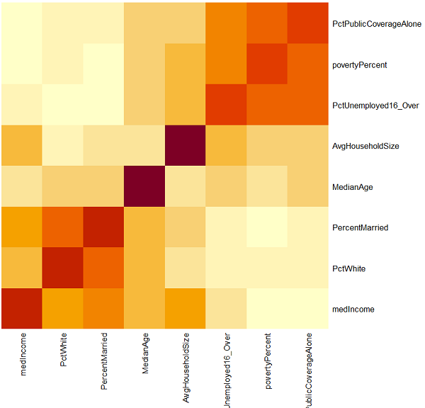
(I trimmed the default dendogram before saving the image.)
Note: a number of correlations are high, most (21/28) were statistically significant (P-value requested, use the Adjusted p-values because of the multiple comparisons problem (see Chapter 12.1).
c.
lm(formula = TARGET_deathRate ~ Region + AvgHouseholdSize + MedianAge +
medIncome + PctPublicCoverageAlone + PctUnemployed16_Over +
PctWhite + povertyPercent, data = cancer_reg)

Coefficients:
                      Estimate Std. Error t value Pr(>|t|)
(Intercept)             158.88      7.387  21.510 < 2e-16 ***
Region[T.North.East]     -2.98      1.763  -1.688 0.0916 .
Region[T.South]           5.35      1.070   4.997 0.000000616 ***
Region[T.West]          -20.80      1.382 -15.051 < 2e-16 ***
AvgHouseholdSize         -2.21      1.018  -2.171 0.0300 *
MedianAge                -0.01      0.009  -0.116 0.9074
medIncome                -0.001     0.001  -4.053 0.000051933 ***
PctPublicCoverageAlone    1.08      0.125   8.662 < 2e-16 ***
PctUnemployed16_Over      1.50      0.176   8.539 < 2e-16 ***
PctWhite                  0.08      0.034   2.439 0.0148 *
povertyPercent           -0.04      0.155  -0.259 0.7953
---
Signif. codes: 0 '***' 0.001 '**' 0.01 '*' 0.05 '.' 0.1 ' ' 1

Residual standard error: 22.79 on 3036 degrees of freedom
Multiple R-squared: 0.3279, Adjusted R-squared: 0.3257
F-statistic: 148.1 on 10 and 3036 DF, p-value: < 2.2e-16

Anova Table (Type II tests)

Response: TARGET_deathRate
                        Sum Sq   Df  F value Pr(>F)
Region                  204634    3 131.3497 < 2.2e-16 ***
AvgHouseholdSize          2447    1   4.7111 0.03005 *
MedianAge                    7    1   0.0135 0.90740
medIncome                 8529    1  16.4232 0.00005193 ***
PctPublicCoverageAlone   38965    1  75.0320 < 2.2e-16 ***
PctUnemployed16_Over     37865    1  72.9130 < 2.2e-16 ***
PctWhite                  3089    1   5.9483 0.01479 *
povertyPercent              35    1   0.0673 0.79529
Residuals              1576628 3036
Besides the intercept, five of seven predictor variables statistically significant. The model R2 is low, 24%; low, but given that the model is about mortality from cancer, explaining 24% of the variability in outcomes from income and other socioeconomic factors is a potentially important result.
Run stepwise regression, criterion = AIC
stepwise(LinearModel.2, direction='backward/forward', criterion='AIC')
Look for best model, at end of the output
The best model, with AIC=19058.43; recall that in general, we favor models with lower AIC values so when you compare your models that’s an acceptable way to select among similar models.
TARGET_deathRate ~ 157.69 - 2.99 Region[T.North.East] + 5.31 Region[T.South] - 20.82 Region[T.West]
- 2.34 (AvgHouseholdSize) - 0.01 (medIncome) + 1.07 (PctPublicCoverageAlone) + 1.49 (PctUnemployed16_Over)
+ 0.87 (PctWhite)
d. Check for multicollinearity. Now that we have our best model, run linear model again, then check VIF.
> vif(LinearModel.3)
                           GVIF Df GVIF^(1/(2*Df))
Region                 1.446657  3   1.063476
AvgHouseholdSize       1.106616  1   1.051958
medIncome              2.450779  1   1.565496
PctPublicCoverageAlone 3.057630  1   1.748608
PctUnemployed16_Over   2.077901  1   1.441493
PctWhite               1.516517  1   1.231470
I ran this through R Commander, therefore vif() command in package car was used. GVIF stands for generalized variance inflation factor is closest to what we traditionally call simply the VIF; the second term GVIF^(1/(2*Df)) . The latter adjusts for the degrees of freedom of categorical (factor) variables. Because we included Region, a factor variable with four levels, we use GVIF^(1/(2*Df)), which makes each term comparable.
When VIF is one, the predictor variables are independent; if VIF is 2, then multicollinearity inflates the variance (standard errors of the coefficients) by a factor of 2. Large VIF indicates presence of multicollinearity: because VIF are less than 2 we would conclude that the four predictors are mostly independent of each other.
The classic formulation of VIF is available in DAAG package.
> DAAG::vif(LinearModel.3, digits=5)
                           VIF
Region[T.North.East]    1.2051
Region[T.South]         1.6336
Region[T.West]          1.3247
AvgHouseholdSize        1.1066
medIncome               2.4508
PctPublicCoverageAlone  3.0576
PctUnemployed16_Over    2.0779
PctWhite                1.5165
/MD