Part 09: Making a report
Instructions on this page are general to use of R and apply to R used on local computer or to users of R in Google CoLab.
Learning objectives
- Create reproducible PDF reports using Markdown and RMarkdown.
- Edit and customize report content within a markdown document.
- Render and export reports efficiently from R script editor, R Commander, or Google CoLab.
What’s on this page?
- Reports and RMarkdown
- How to generate a report
- What R code do I submit?
- Some basic Markdown
- Generate the report
- To do on your own
- Quiz
What to do
Work through the examples to learn how create and generate reports for your homework within R Commander or even just the built-in R script editor. Although you can copy/paste to a word document, insert images, edit, then save to a pdf, this is an inefficient and error-prone process. Far better to struggle a bit to learn RMarkdown and a work flow like the one presented on this page; the benefits later with more challenging homework will be worth the effort.
For those of you working with Google CoLab, generating a report is straightforward. You’ve already learned how to start and enter code via the + Code button; for text, simply click + Code button in the CoLab toolbar and add your notes or responses to homework questions. Then, simply save to pdf file your code, text, equations, and executed R outputs/plots by submitting the page to your browser Print Save as PDF option.
How to do it
For these exercises, you may work
- within the Rcmdr script window
- RStudio
- Google CoLab
- Built-in R scripte editor
Choose one way. The quickest way is to just work with R Commander, but RMarkdown was designed to work with RStudio.
Markdown and Jupyter Notebooks, like those used in Google CoLab, work well together.
Let’s begin.
1. Reports and RMarkdown
An important component of your work in this class is to make reports detailing your results. Now, we don’t want you to submit all of your script attempts, just the last edited versons that address the questions and results necessary to complete your homework. Especially early on, it’s easy to generate lots of code — thus, you’d be expected to edit out all of the practice runs leaving only the relevant useful code and R output.
Moreover, we ask that homework be submitted as pdf reports. PDF files have the advantage that they maintain formatting so that documents appear the same on any device. Importantly for homework, pdf documents are harder to manipulate compared to Word documents. Pdf documents maintain the integrity of homework.
Thus, it is an important skill to learn in our biostatistics class how to generate pdf reports from your work. Your first instincts may be to copy and paste your work from R into a word document, then generate a pdf — and you have likely done this many times before. However, this is a time consuming and error-prone work flow — I want you to learn the advantages of Markdown when creating technical reports.
Note 1: Markdown, not R Markdown, is default in any Jupyter Notebook, including Google CoLaboratory. For Google CoLab users, where this text reads “RMarkdown,” assume the statements apply to you. The folks at RStudio have come up with an even better system called Quarto, but this page does not address use of that system.
Markdown is a hugely important innovation. While you can copy and paste your work from R output to Word document — which is something we used to do — the advantage of RMarkdown is it preserves your code. In practice then, you can run code from a Markdown Report — an advantage for producing reproducible code. RMarkdown helps us avoid this copy/paste step to a different app, and does much better at preserving the work we do in R, as you will quickly learn if you try and rely on the copy/paste route!
R Commander (and RStudio) use RMarkdown, which does a great job of capturing and presenting your work with a minimum of effort. (Yes, you can accomplish the same using only a script editor, (click here for markdown use of R script editor.)
Note 2: RMarkdown is a version of Markdown, a markup language to help you create formatted text using a plain-text editor (see Wikipedia). RMarkdown is a dynamic document format that combines Markdown text with chunks of executable R code.
CoLab, skip this step. In R Commander, once you are ready to generate a report, click on the R Markdown tab (blue arrow) to bring up the Markdown text window (Fig 1).
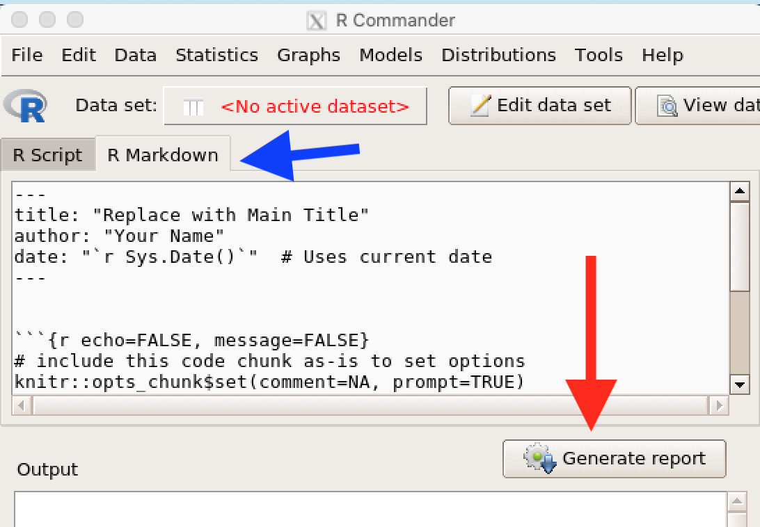
Figure 1. R Markdown text window.
Mix R code and text in one document.
The Rmd document begins with some YAML metadata. Figure 1 shows
---
title: "Replace with Main Title"
author: "Your name"
date: "'r Sys.date()'"  # Uses current date
---
YAML (which stands for YAML Ain’t Markup Language) is a simple text format used to store configuration settings. In R Markdown, it sits at the very top of your document between two sets of triple dashes (—). It acts as the control panel or metadata for your file, telling R studio crucial information like title, date, authorshio, along with other document settings.
The advantage of rmarkdown is that you can mix text and R code. Text entered can be formatted with simple markdown code (see below), but code chunks are bracketed by
'''{r}
your code here
'''
When you submit the .Rmd file, R renders the code and embeds the output along with your entered text.
Note 3: Note the curly brackets around r.
``` r tells the compiler: “Display this text.”
```{r} tells the compiler: “Open up a live R environment, load this command, and inject the results directly into the HTML file.”
2. How to generate a report
CoLab, skip this step. Good practice tip: When you first open R Commander (click here for use of R script editor only), click on the R Markdown tab and replace title: and author: with a descriptive title for your report and your name (leave the quotes) (Fig 1).
---
title: "My homework"
author: "Keoni Kahele"
---
Then, click on the R Script tab and proceed with work on your project or homework.
Note 4: Keoni Kahele is my attempt at “John Doe,” with assistance from Gemini and ChatGPT along with references to Glosbe. Keoni is traditional Hawaiian transliteration equivalent of the English name “John”. Kahele is a common Hawaiian surname meaning “the walk” or “the moving”. I elected not to go with Keoni Kō because of it’s negative connotations to many in Hawai’i, see Keoni Kō, Pala ka Mai‘a by Kīhei de Silva at Ka’iwakīloumoku.
At the conclusion of your work, click on the R Markdown tab and scroll through your text. You can delete or add text as you please. To retain R commands and output, just don’t edit anywhere between ```{r} and ```
```{r}
some R command here
```
making changes to the markdown template (eg, adding additional text to answer questions, etc.), then click Generate report (Fig 1, red arrow).
And if you’re not using R Commander or RStudio? Yes, you can generate a rmarkdown report file with just the R script editor. You need to load the following three packages
- knitr
- markdown
- rmarkdown
Start the R script editor. Our goal is to generate an html page and load it to our default browser (eg Chrome or Safari). From there, simple enough to print to a pdf file.
Select File > New script (on Windows) or File > New Document (on macOS).
Paste the minimal R markdown template, the yaml metadata, into the empty script:
---
title: "Homework 2B"
author: "Keoni Kahele"
---
Add your R work as needed. For example, Question 2 of Homework 2B asks to calculate mean, median, and mode for y <- c(1,1,3,6) . To the script we add
### Question 2
```{r}
y <- c(1,1,3,6)
mean(y)
median(y)
temp = table(as.vector(y))
names (temp)[temp==max(temp)]
```
The mean was 2.8, median was 2, and mode was 1.

### End homework
Save this script to your working folder, eg YourName_Hwk2B.Rmd.
Back at the R prompt, enter the following code
output_path <- knit2html("myR-code.Rmd")
browseURL(output_path)
Note 5: Best practice — call the file by name (and path, if not in working folder) directly. When calling for R to load a file, I frequently use file.choose() rather than writing the file name. This works fine provided the call is not in a code chunk inside the R Markdown document itself; doing so will fail to render or knit2html because the background processes fail to open popup windows and will crash with file choose cancelled error message.
Your browser opens up with your new html file (Fig 2).
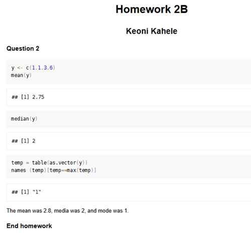
Figure 2. Screencapture of html output file from Rmarkdown.
Note 6: knit2html() is not the modern route. A better option would be to use render(), which is part of the rmarkdown package.
output_path <- render("myR-code.Rmd", output_format = "html_document")
Among the advantages, take full advantage of yaml metadata formatting. For example, we can add a simple table of contents to our document:
---
title: "Homework 3"
author: "Keoni Kahele"
output:
html_document:
toc: true
toc_float: true
---
The result? Our formatted html document but with a table of contents right after “author,” complete with hyperlinks to the questions, which we set to heading 3 (###).
What R code do I submit?
For your projects, it is a good ideaa to provide your code as an appendix. For a homework, typically we do not want you to submit copied R code that was provided to you. In your rmardkwn file, identify the code chunk, then, hide the code, but show the output (echo = FALSE). For example,
```{r setup, echo = FALSE}
# This code runs and its results/plots will show,
# but the code itself is completely hidden in the final report.
library(ggplot2)
print("This text/output will show, but this code won't!")
```
Use this when the provided code generates a plot, table, or calculation that you need to display for your homework, but you don’t need to share the raw R script with the instructor.
3. Some basic Markdown
While you can copy/paste from R output to Google Doc or MS Word, I want you to use RMarkdown to craft your responses to homework. RMarkdown captures your script and R output in one form; it is simple to insert your own text. The result is a single organized document.
I do expect you to remove “mistakes” (incorrect function calls because of typos, etc.,) from your R Markdown text before you generate a report. Once an .Rmd file has been created, open it in your favorite text editor (TextEdit, Notepad). Your work will look better if you apply a bit of Markdown syntax. Alternatively, you can use html syntax — Markdown is just simple text. While you can do all of the edits you need within the Rcmdr editor, many useful Markdown editors available (eg, PanWriter, MarkText), which makes working with Markdown files simple once you get used to looking at the markdown language.
Note 7: RMarkdown includes formatting not part of the basic Markdown language; neither PanWriter nor MarkText perserve RMarkdown edits.
Really, to make an elegant report, all the “markdown” you need is how to include headings. In html-CSS, headings are coded with tags (Table 1).
Table 1. html-css tags with markdown equivalents
| html tag | markdown | description |
| <h1> some text </h1> | # some text |
primary (main) heading 1 |
| <h2> some text </h2> | ## some text |
subheading 2 |
| <h3> some text </h3> | ### some text |
subheading 3 |
| <h4> some text </h4> | #### some text |
subheading 4 |
| <h5> some text </h5> | ##### some text |
subheading 5 |
| <h6> some text </h6> | ###### some text |
subheading 6 |
the basics you need to know are
- code blocks
- headings
- insert image
- lists (ordered and numbered)
We’ll improve with markdown as the semester unfolds, but I recommend you start with one of many free online tutorials, eg, https://www.markdowntutorial.com/
Here, I’ll step you through a mock homework. The mock homework questions
CoLab, skip this step. Question 1. When you exit R and Rcmdr, you are prompted to save a number of files. Make two lists: files exit from Rcmdr, files exit from R.
Note 8: If you recall, I’ve instructed that for general use by students, none of these files should be saved from an R session.
CoLab, skip this step. Question 2. Which file(s) capture all of your work, including mistakes?
Hint: See Part 10: Exiting R and Rcmdr
Question 3. Load the dataset DNase (package dataset) and make a scatterplot of density by conc, include by groups.
Here’s my markdown script. Text I entered into the markdown script file marked in yellow.
---
title: "Part 09: Making a report"
author: "Keoni Kahele"
date: "`r Sys.Date()`" # Uses current date
---


```{r echo=FALSE, message=FALSE}
# include this code chunk as-is to set options
knitr::opts_chunk$set(comment=NA, prompt=TRUE)
library(Rcmdr)
library(car)
library(RcmdrMisc)
```


```{r echo=FALSE}
# include this code chunk as-is to enable 3D graphs
library(rgl)
knitr::knit_hooks$set(webgl = hook_webgl)
```

### Question 1

#### Exit Rcmdr only

1. script file
2. R Markdown file
3. Output file

#### Exit R
1. Workspace image

### Question 2

Workspace image. Available in .Rhistory

### Question 3

```{r}
data(DNase, package="datasets")
```

```{r}
scatterplot(density~conc | Run, regLine=FALSE, smooth=FALSE, boxplots=FALSE,
by.groups=TRUE, data=DNase)
```

### End of report
The rendered document from this markdown script is shown in Figure 3. Heads up: I used html (<h3>, <p>) and Markdown (ordered list). Importantly, the simple way to hide R function calls, just a little markdown code
```{r echo=FALSE}
above the command hides the command, whereas
```{r}
ensures that the commands are printed.
Note 9: It helps to add space before and after ### and text blocks so that they render properly. Results look like Figure 3 below.
I do encourage you to explore Markdown — it’s really handy and simple to learn. You can use the editor included in Rcmdr (or RStudio, which is really nice for generating markdown reports), or you can copy the script into your favorite text editor (eg, Notepad, TextEdit), make your changes, then copy back to Rcmdr before rendering. See https://en.wikipedia.org/wiki/Markdown#Example for some suggestions. A nice tutorial is available at https://www.markdowntutorial.com/.
4. Generate the report
Submit homework in BI311 as pdf files. The expectation is that you work with RMarkdown.
If you did not install the auxillary tools LaTeX and pandoc, then the default use of generatign the report will return an html file suitable for viewing in your browser.
For full function, pandoc and LaTeX installed on your computer is recommended. Check by clicking on Rcmdr: Tools > and look for a submenu choice: Install other software (if you don’t see this option it means you already have pandoc and LaTeX available on your computer).
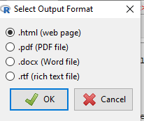
Figure 2. Screenshot of format options available for a computer with working LaTex and pandoc.
Note 10: This message is for those of you who have successfully installed R and are running R Commander, but may be having problems installing pandoc or LaTeX. While there’s some advantage to getting pandoc etc working, it is not essential for BI311 work. Assuming you have Rcmdr and RcmdrMisc installed, and if you have started Rcmdr and have it up and running, then we can skip pandoc and LaTeX installation and use features of your browser to save to pdf.
R Markdown by default will print to a web page (an html document called RcmdrMarkdown.html) and display it in your default browser. To meet requirements of BI311 — you submit pdf files — we can print the html document generated from “Generate Report” in R Commander to a pdf.
- Chrome browser, right click in the web page, from the popup menu select Print, then change destination to Save as pdf.
- Safari browser, right click then select Print page (or if an option, Save page as pdf), then find at lower left find PDF and option to Save as PDF.
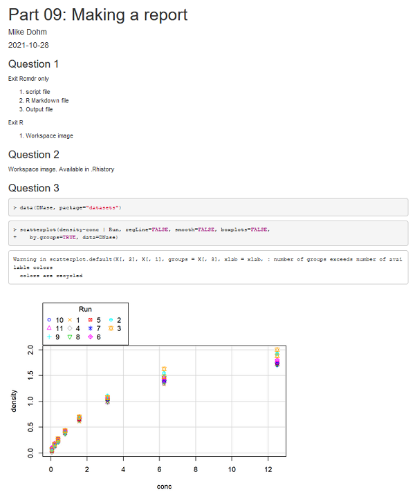
Figure 3. Screenshot of rendered RMarkdown script for the mock homework.
5. To do on your own
Repeat my mock homework to confirm you can generate a markdown file that looks like mine.
Select work done from any one (or more) of the lessons on R and R Commander, make an R Markdown report, and export as a pdf file.
Part 04. Create functions in R
Part 05. R packages: Making R do more
Part 06. Work with an included dataset
Part 07. Working with your own data
6. Page quiz
draft, more questions soon
Reports
Five questions from this page