Answers: Correlation and simple linear regression

Homework 9: Correlation and simple linear regression

Answers to selected number problems

Answers to selected problems

Part 1

1.
install.packages("MASS")
library(MASS)
data(Animals, package="MASS")

classType <- c("M","M","M","M","M","D","M","M","M","M","M","M","M","H","M","D","M","M","M","M","M","M","M","M","M","M","D","M")
dAnimals <-data.frame(classType,Animals)
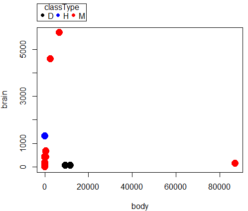
scatterplot(brain~body | classType, regLine=FALSE, smooth=FALSE, by.groups=TRUE, pch=c(19,19,19), cex=c(2,2,2), col=c("black", "blue", "red"), grid=FALSE, data=dAnimals)

3. 
normalityTest(~brain, test="shapiro.test", data=Animals)

Shapiro-Wilk normality test

data: brain
W = 0.45173, p-value = 0.000000003763

Clearly, we reject null hypothesis, “brain” not normally distributed.

normalityTest(~body, test="shapiro.test", data=Animals)

Shapiro-Wilk normality test

data: body
W = 0.27831, p-value = 1.115e-10

Clearly, we reject null hypothesis, “body” not normally distributed.

Rcmdr: Statistics → Summaries → Correlation test

with(Animals, cor.test(body, brain, alternative="two.sided", 
+ method="spearman"))

Spearman's rank correlation rho

data: body and brain
S = 1036.6, p-value = 0.00001813
alternative hypothesis: true rho is not equal to 0
sample estimates:
rho 
0.7162994

Question 1. Parametric tests involve estimation of population parameters, e.g., correlation between body weight of “mammals” and brain weight of “mammals”. Parametric statistics require certain assumptions hold, for example, normality. Nonparametric tests test similar hypotheses, but do so on ranks, not the original data. Thus, fewer assumptions are made about the quality of the data as no effort is made to infer population parameter values.

Question 3. Spearman rank correlation (0.716, P = 0.000018) is best and we conclude there is a positive association between brain and body weight in this sample of mammal species. Note that the Pearson product moment correlation was small and negative (-0.0053), and not statistically different from zero (P = 0.979). However, we can’t trust this estimate because the assumption of normality was clearly violated for both these variables (brain weight: p-value = 0.000000003763; body weight: p-value = 1.115e-10. See normality test #5 above).

Part 2

1. There are just two variables. “speed” is clearly an independent variable whereas “dist” (stopping distance) is the dependent variable.
2. scatterplot

3. histogram

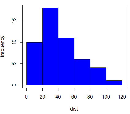
4. dist, Shapiro-wilk p-value = 0.0391

Question 1. Because we reject normality assumption for dist, we log10-transform dist to create new variable, lgDist. However, lgDist is even less normally distributed (Shapiro-Wilk normality test p-value = 0.001066), we conduct our linear regression test of speed on untransformed dist.

Results were

lm(formula = dist ~ speed, data = myData)

Residuals:
Min 1Q Median 3Q Max 
-29.069 -9.525 -2.272 9.215 43.201

Coefficients:
Estimate Std. Error t value Pr(>|t|) 
(Intercept) -17.5791 6.7584 -2.601 0.0123 * 
speed 3.9324 0.4155 9.464 1.49e-12 ***

Residual standard error: 15.38 on 48 degrees of freedom
Multiple R-squared: 0.6511, Adjusted R-squared: 0.6438 
F-statistic: 89.57 on 1 and 48 DF, p-value: 1.49e-12

Rcmdr: Models → Hypothesis tests → ANOVA table

Anova(LinearModel.3, type="II")
Anova Table (Type II tests)

Response: dist
          Sum Sq  Df   F value    Pr(>F) 
speed      21186   1    89.567  1.49e-12 ***
Residuals  11354  48

6.
a) b₀ (Y-intercept) = -17.5791
b) Null hypothesis: Y-intercept equals zero. P-value = 0.0123, therefore we reject null hypothesis
c) b₁ (slope) = 3.9324
d) Null hypothesis: slope equals zero. P-value = 1.49e-12, therefore we reject null hypothesis
e) dist = -17.5791 + 3.9324(speed)
f) Adjusted R-squared: 0.6438

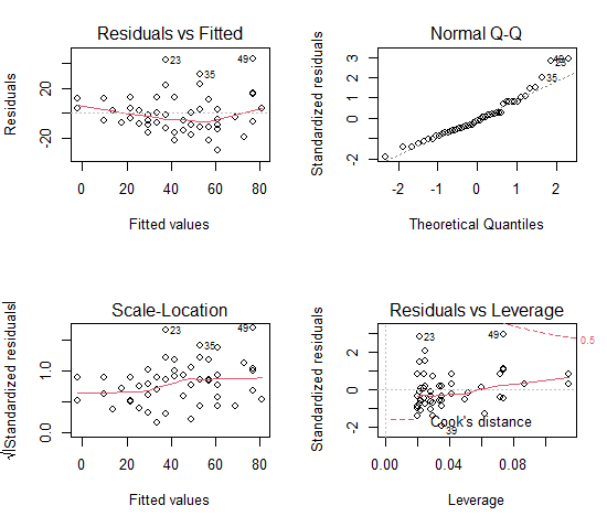
Top-left graph: No obvious trend in residuals

Top-right graph: Q-Q plot suggests some deviation from normality (points 25, 35, 49), which is consistent with our test of normality

Bottom left graph: some trend in variances; increases with increasing fitted (predicted) values

Bottom right graph: No evidence of influence point (no data outside Cook’s distance, see dashed red line)

Numerical diagnostics: Only numerical test appropriate is Breusch-Pagan test of variance of errors normally distributed (no heteroscedasticity)

Breusch-Pagan test

data: dist ~ speed
BP = 4.6502, df = 1, p-value = 0.03105

Question 3. We conclude that our simple model, knowing speed of the car, explains 64% of variance in stopping distance. Some indications that distance not normally distributed and a possible pattern in residuals (BP test significant for heteroscedasticity), which may warrant additional addition.