Homework 5: Inference
Homework objectives
- Explore null and alternate hypothesis concepts.
- Explain relationship between outcomes of a test of hypothesis and interpretation of a diagnostic test result.
- Evaluate error rates (Type I, Type II) and critical value, p-value.
Homework 5 expectations
BI-311 students: For homework reports, report only your answers for the even numbered questions. Read through the entire homework before starting to answer a question — all questions are intended to help you achieve the learning outcomes for the chapter. You are expected to have read the chapter and to have completed preceding homework. Answers are provided to odd numbered problems — turn in your work for even numbered problems.
How to work this homework
You may work together, but each of your must turn in your own report. Don’t “plagiarize” from each other. Do include in your report who you worked with.
What to turn in: A pdf file containing your answers to the even-numbered questions and relevant R code; by relevant we mean include your code, not copies of code provided to you. For statistical results, report appropriate significant figures. Use of RMarkdown recommended — because it is a simple way to include graphs generated; however copy/paste into a word document, then converted to pdf, is also acceptable.
Note 1: By relevant we mean provide just the R code and results from R functions necessary to support your answers to the questions. For example, do not include
- my code; if you’ve modified my code, then include just your modifications, not the whole code — which was given to you 😉
- the entire data set when
head(dataset)will do - screenshots of R output!!
- R output is just text — edit your work in markdown
- If you do not use markdown, instead employing copy/paste — that’s OK, but edit your work
- all statistical output from an R function.
- Be selective! Include what is needed to answer the question.
See Part09: Making a report for an example homework file.
Submit your work to CANVAS. Obey proper file naming formats.
Resources for this homework
Chapter 8. Mike’s Biostatistics Book
Mike’s Workbook for Biostatistics: A quick look at R and R Commander, Part01 – Part10 and previous homework pages presented in this workbook.
Additional R commands and or code provided below.
Questions
1. Match the four (shaded) corresponding cells in the two tables. For example, which outcome from the Table 1 matches specificity of the test in Table 2? Repeat for all four cells
Table 1. When conducting hypothesis testing, four outcomes are possible.
| HO in the population | |||
| True | False | ||
| Result of statistical test | Reject HO | Type I error with probability equal to α (alpha) |
Correct decision, with probability equal to 1 – β (1 – beta) |
| Fail to reject HO | Correct decision with probability equal to 1 – α (1 – alpha) |
Type II error with probability equal to β (beta) |
|
Table 2. Interpretations of results of a diagnostic or clinical test.
| Does the person have the disease? | |||
| Yes | No | ||
| Result of the diagnostic test |
Positive | a
sensitivity of the test |
b
False positive |
| Negative | c
False negative |
d
specificity of the test |
|
2. Find three sources on the web for definitions of the p-value. Write out these definitions in your notes and compare them.
3. In your own words distinguish between the test statistic and the critical value.
4. Can the p-value associated with the test statistic ever be zero? Explain.
5. We provided a table of some incorrect interpretations of NSHT p-values:
- the probability of obtaining the observed data under the assumption of no real effect
- an observed type-I error rate
- the false discovery rate, i.e. the probability that a significant finding is a “false positive”
- the (posterior) probability of the null hypothesis.
With the p-value interpretations listed in the table above in hand, select a research article from PLoS Biology, or any of your other favorite research journals, and read how the authors report results of significance testing. Try a variety of search strategies.
For example, I searched an article for the following terms
null, 0
significant, 13
significance, 2
For the latter, the phrase “Asterisks indicate statistical significance” referred to a figure, and I couldn’t find any definition for what the authors meant by statistical significance. The most likely interpretation would be item 1 from our table.
Your objective is to compare the precise wording in the results section against the interpretative phrasing in the discussion section. Do the authors fall into any of the p-value corner-cutting traps?
6. For a Type I error rate of 5% and the following degrees of freedom, compare the t-distribution critical values for one tail test and a two tailed test of the null hypothesis.
- 5 df
- 10 df
- 15 df
- 20 df
- 25 df
- 30 df
Using your findings, make a scatterplot with degrees of freedom on the horizontal axis and critical values on the vertical axis.
What trend do you see for the difference between one and two tailed tests as degrees of freedom increase?
7. You open up a bag of Original Skittles and count the number of green, orange, purple, red, and yellow candies in the bag. What kind of hypothesis should be used, one-tailed or two-tailed? Justify your choice and sketch out the null and alternative hypothesis.
8. A clinical nutrition researcher wishes to test the hypothesis that a vegan diet lowers total serum cholesterol levels compared to an omnivorous diet. What kind of hypothesis should he use, one-tailed or two-tailed? Justify your choice and sketch out the null and alternative hypothesis.
9. Spironolactone, introduced in 1953, is used to block aldosterone in hypertensive patients. A newer drug eplerenone, approved by the FDA in 2002, is reported to have the same benefits as spironolactone (reduced mortality, fewer hospitalization events), but with fewer side effects compared with spironolactone. Does this sentence suggest a one-tailed test or a two-tailed test? Justify your choice and sketch out the null and alternative hypothesis.
10. Output from a one-sample t-test for body weights of lizards was presented in this Chapter. The R output is shown below
One Sample t-test
data: lizards$Body.mass
t = -1.5079, df = 7, p-value = 0.1753 alternative hypothesis: true mean is not equal to 5
95 percent confidence interval:
2.668108 5.515892
sample estimates:
mean of x
4.092
Answer the following questions
10a. Was this a one-tailed or two-tailed hypothesis test?
10b. Write out the null hypothesis
10c. What was the value of the test statistic?
- -1.5079
- 7
- 0.1753
- 2.668108
- 5.515892
- 4.092
10d. What was the P-value?
- -1.5079
- 7
- 0.1753
- 2.668108
- 5.515892
10e. We should reject the null hypothesis
- False
- True
10f. Write out the interpretation of the hypothesis test as we would in a research article.
11a. To gain practice with calculations of confidence intervals, calculate the approximate confidence interval, the 95% and the 99% confidence intervals based on the t distribution, for each of the following.
![\[\bar{X} = 13, s = 1.3, n = 10\]](https://mikeworkbook.letgen.org/wp-content/ql-cache/quicklatex.com-d0aaa1307540ee229a31f288de0708d0_l3.png "Rendered by QuickLaTeX.com")
![\[\bar{X} = 13, s = 1.3, n = 30\]](https://mikeworkbook.letgen.org/wp-content/ql-cache/quicklatex.com-4a69bbda92e4479c00e180b2c767a751_l3.png "Rendered by QuickLaTeX.com")
![\[\bar{X} = 13, s = 2.6, n = 10\]](https://mikeworkbook.letgen.org/wp-content/ql-cache/quicklatex.com-aebc6e25c57cc08e9798f8bf92afb28e_l3.png "Rendered by QuickLaTeX.com")
![\[\bar{X} = 13, s = 2.6, n = 30\]](https://mikeworkbook.letgen.org/wp-content/ql-cache/quicklatex.com-cd90c377cb616acbfc6c5dac3cfb6a62_l3.png "Rendered by QuickLaTeX.com")
11b. Take at look at your answers to question 11a — what trend(s) in the confidence interval calculations do you see with respect to variability?
11c. Take at look at your answers to question 11a — what trend(s) in the confidence interval calculations do you see with respect to sample size?
R or Rcmdr commands
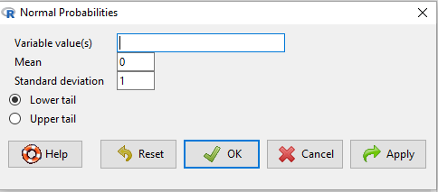
Work Z-score problems
Rcmdr: Distributions → Continuous distributions → Normal distribution → Normal probabilities …
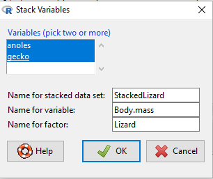
Stack variables
Rcmdr: Data → Active data set → Stack variables in active data set…
gecko <- c(3.186, 2.427,4.031,1.995)
anoles <- c(5.515,5.659,6.739,3.184)
lizard <- data.frame(gecko,anoles)
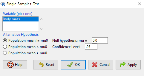
One sample t-test
Rcmdr: Statistics → Means → Single-sample t-test…
Type I error rate, calculate the degrees of freedom (df), and lookup the critical t value from the table
one tail critical value, eg, seven degrees of freedom
qt(c(0.05), df=7, lower.tail=FALSE)
two-tail critical value, eg, seven degrees of freedom
qt(c(0.025), df=7, lower.tail=FALSE)
Or, use Rcmdr instead
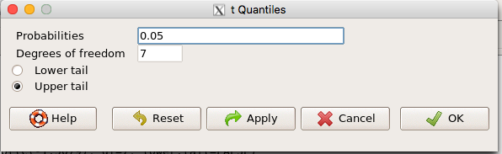
Rcmdr: Distributions → Continuous distributions → t distribution → t quantiles…
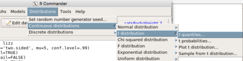
enter the alpha level (Probabilities), the degree of freedom, and check the tail
/MD