Part 02. Getting started with R and Rcmdr

This page is primarily about use of R Commander and local installation of R. However, there are also instructions about project management that apply to users of R in Google CoLab.

Learning objectives

• Set and change the working directory in R session to organize your project files effectively for course-based analyses.
• Start and stop R and R Commander (Rcmdr) properly, ensuring a smooth workflow using the R Commander script interface.
• Understand how to navigate R Commander’s interface—working with menus, script window, output, and messages panes—to structure your coding and analyses clearly.

What’s on this page?

A lot! Scan a topic, pick and choose. The goal was to provide lots of “how tos” and you would return as “how do I…” questions arise.

1. Project management — Prepare your computer
2. Start R
3. Start R Commander
4. Stop, exit, quit current R session
5. Identify Working folder in R
6. Change Working folder in R
7. Access and use R GUI script window
8. R Commander windows
9. Call system commands (optional)
10. References and suggested readings
11. Quiz

A reminder to Google CoLab (serverless computer) users: the page is written assuming the reader runs a local installed R environment, not a serverless computing environment like CoLab. However, specific CoLab instructions are included where relevant and, if the code does not apply to CoLab, then the text begins with CoLab, skip this step statement.

What to do

First, decide which coding environment you will use for the semester. Your options include

1. R Commander with the Rcmdr script window.
2. R GUI app, code entered and run from a script document.
3. RStudio.
4. R GUI app, commands entered at the command line and R prompt.
5. Google CoLab or other cloud service.

For more about this choice, see A quick look at R and R commander in Mike’s Biostatistics Book.

How to do it

My recommendation for BI311 students, option 1 is the way to go (see justification Why R Commander in Mike’s Biostatistics Book). We are starting from the perspective that your experience with R to date is minimal. RStudio is the choice for coding and managing statistical projects; however, it’s way more IDE for beginners with statistics. Although R Commander will work within R Studio, the experience is not great. Thus, R and R Commander or R and RStudio, but not R plus RStudio plus R Commander.

This page is about working with R and R Commander together. Learn how to start and stop R and R Commander. Setup your environment, which is the foundation for project organization. Introduce the idea of writing code as script. There’s also some code to explore how to call system commands from within R. Operating specific code is provided. Wikipedia links to common computer terms are provided.

If running R with Google CoLaboratory, then the look and feel of the Jupyter Notebook interface is quite different, but logical and easy to learn. The basics — select the +Code button to add a code box and select the +Text button to add comments or answer homework questions. To run a command, click the “Run cell” button.

CoLab, skip this step. As a reminder, to run or submit an R command from the command line in R (denoted by the R prompt “>”), press the enter or return key. To run a command or series of R commands in a script file, highlight the line(s), then press one after the other Ctrl+r (WinPC). If macOS, then the same function is via key press Cmd+return. R Commander provides a “Submit” button that works like Ctrl+r and Cmd+return key press.

1. Project management — Prepare your computer

To do before starting R

1. We want you to get into the habit of setting working folders.
   • So if you have not already done so, set up a working folder (e.g., BI311) and make it available in R.
   • Practice using getwd() and setwd().
2. Use Sys.getenv() to locate where on your computer R is installed.
3. Optional, explore use of system commands within R to move around on your computer.

What is a working folder?

During the semester you’ll be working on a number of projects. Some projects will have a few files, others may have dozens of files. It’s therefore good practice — a basic data management skill — to apply project organization principles: Set up and use a folder/file structure for your work in the course.

Google CoLaboratory users, see Help with Google CoLab environment.

CoLab, skip this step. The steps described here show you how to change your working folder for an R session. Once you end the session (e.g., exit R), then the next time you start R, you’d have to repeat these steps to change your working folder. I prefer this approach because I work with many different R projects, so I have working folders for each project, and use scripts which include steps to change to the preferred working folder. However, you may prefer to make the working folder the default choice. You can do this by editing a text file called .RProfile. How to edit this file is described in the Optional: Modify .RProfile page.

Setup a working folder on your computer

The concept of a working folder applies to both the serverless computing environment and a local R environment. For Google CoLab, mount your Google Drive and point to a folder in My Drive. See Help with Google CoLab environment. in this workbook and Mike’s Biostatistics Book — Use R in the cloud.

CoLab, skip this step. Create a folder on your computer to hold all of your R work. For example, it might be something like “BI311” as a subfolder on your Desktop or in your Documents folder. Note that USERNAME would be specific to your computer; replace “BI311” with the name of your working folder.

On a Mac, the path to BI311 off the Desktop would be

/Users/USERNAME/Desktop/BI311

You can copy the path as displayed to R in the next step (Identify Working Folder in R).

• macOS tip: Want to quickly view the Desktop? Keyboard shortcut Cmd+F3 or Fn+F11 will work.
• macOS tip: To view the path, Finder → View → Show Path Bar (keyboard shortcut Alt+Cmd+P).

MacOS readers, you’re good to go. Skip down to Start R.

Win11 readers, we have a little work to do, so begin. On a Win11, the path to BI311 off the Desktop would be

C:\Users\USERNAME\Desktop\BI311

You can copy the path as displayed to R in the next step (Identify Working Folder in R).

• Win11 tip: Want to quickly view the Desktop? Keyboard shortcut Windows key ⊞ +D
• Win11 tip: To view the path, File Explorer → View → Options → Change folder and search options → View → Display the full path in the title bar (check the box)

Win11 uses “\” (backward slash), not “/” (forward slash) like macOS — and everyone else in the computer world! A long time ago, Microsoft chose to go against the forward-slash convention, and we’ve been paying for it ever since. We provide a few options (tricks) to get R to help here — see Trick 1 and Trick 2 below.

To R, a backslash is treated as an escape character. Unfortunately, you’ll need to change this. So, either retype the path to replace backslashes with forward slashes

C:/Users/USERNAME/Desktop/BI311

Or, you can use one of the following tricks. Copy the Win11 path to the clipboard, then

Trick 1: write and submit the command in R

setwd(readClipboard())

the readClipboard() function takes the forward slashes and replaces with “//”. Check the directory was changed

getwd()

returns

"C:/Users/USERNAME/Desktop/BI311"

this will work for us without further modification. With the extra backslash our path backslash is not treated as an escape character.

Trick 2: treat the path as a raw string (Hadley et al 2020).

setwd(r"(C:\Users\USERNAME\Desktop\BI311)")

r"" allows you to write the path as a “raw string constant.” h/t Henrik response at stackoverflow.com.

Continue reading — we return to paths when we introduce setting the working folder in R.

2. Start R

MacOS users, the app is simply R.app. Figure 1 displays R session immediately after start, running on macOS.

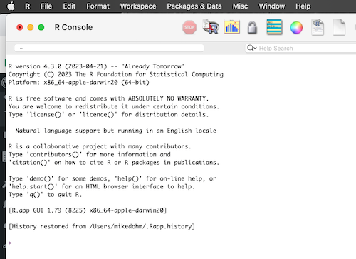
Figure 1. Screenshot of R console at startup of an R session running on macOS.

Win11 users, the app is Rgui.exe. Start as you would any application installed on your computer. If you followed out instructions, then the R icon is likely on your desktop; apps can also be quickly launched by pressing the Windows key to open the search menu, type “R”, and then press the Enter key to launch the R console.

Linux? From the terminal, type and submit R.

To start an R session in CoLab, see Mike’s Biostatistics Book — Use R in the cloud. An R session running in the Google CoLaboratory cloud service is shown in Figure 2.

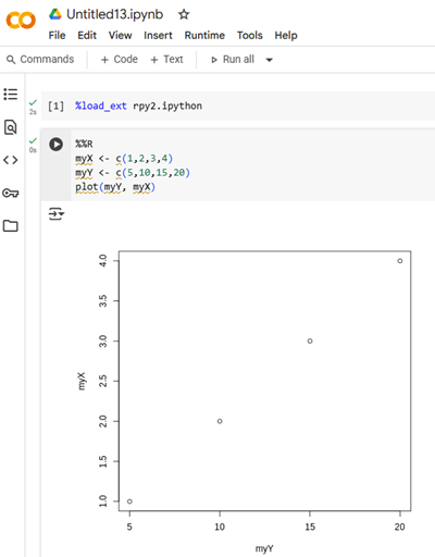
Figure 2. Screenshot of Jupyter Notebook at startup of an R session in Google CoLab.

3. Start script editor

CoLab, skip this step. It is not necessary to run R in RStudio or, for that matter, R Commander. The basic R GUI includes the facility to start, open, and save script files, which is the lifeblood of R coding. With the R app running, on WinPC select File New script (Fig 3).

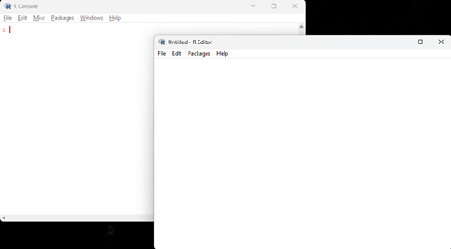
Figure 3. Screenshot of R Console with text editor opened.

However, as of Fall 2025 I continue to recommend that new statistics students run R within R Commander because it provides access to function calls from drop down menus. Off we go.

At the R prompt (the “>” in Figure 1), type

 library(Rcmdr)

R is case sensitive. That means, type exactly library(Rcmdr), not Library(Rcmdr) or library(RCMDR), etc.

4. Stop, exit, quit current R session

Quit, prompt with prompt to save workspace image. For most users just getting started, select Don’t save.

Let’s get to work

You may complete the next work within the standard R work area, or from an R script, or within the R Commander script window. Commands intended to move about your computer obviously won’t work if you’re running R in the cloud (CoCalc or Colaboratory), but other commands will work fine!

From here on I assume you are working in R Commander’s script window. Don’t forget to submit you commands in R Commander (place the cursor at start of the code, then press Submit button).

5. Identify Working folder in R

Now that R Commander is running, let’s get our environment set up.

First, what is the current Working directory (folder)? This is the default location where R will save files (it was established based on choices you made when you first installed R).

Type the function

getwd()

then submit. R will show something like (macOS result)

[1] "/Users/USERNAME/"

Second, change default folder in R to match the working directory you just created. You’ll need to copy the full path to your clipboard.  Skip down to Change Working Folder in R.

Yet another option, check location your R installation (R_HOME) and your current working folder (HOME).

Sys.getenv(c("R_HOME","HOME"))

On my Win11, R returns

>Sys.getenv(c("R_HOME","HOME"))
R_HOME HOME 
"C:/R/R-4.1.0" "C:\\Users\\USERNAME"

On my macOS Catalina, R returns

>Sys.getenv(c("R_HOME","HOME"))
                                     R_HOME 
"/Library/Frameworks/R.framework/Resources" 
    HOME
"/Users/USERNAME"

If you recall our work with forward slash and Win11 paths above, we have an object called myFolder. We can now set the working folder simply by writing and submitting the following code at the prompt

setwd(myFolder)

Alternatively, if you’re running Win11 (this doesn’t work on macOS), I can get help from R with this task. At the R prompt write and submit

choose.dir()

which will bring up Explorer (Windows). You then browse to the folder you created on your desktop. from which you can select the directory (folder) you wish to use (see On Win11 PCs, you can combine setwd() and choose.dir() below).

A related function is file.choose(), but for selecting files, not folders. This function does what it says, it allows you to find and load files into R and it works on both macOS and Win11 PCs. On macs you can use this function much like the choose.dir() command. If you have a file already in the folder, then skip this next suggestion, just use file.choose() to browse to your folder and select a file. If the working folder is empty, then create and save a text file to the folder. For example, I created a text file in TextEditor called justAfile.txt and saved to my working directory. Then, in R

myFolder <- file.choose()

The object myFolder holds the path to justAfile.txt

[1] "Users/USERNAME/Desktop/BI311/justAfile.txt"

Now, just edit the object, remove “justAfile.txt” There’s a variety of ways to do this — the simplest is to just copy/paste into TextEdit and then use the result. Or, you can use the following

myPath <- unlist(strsplit(myFolder, split="justAfile.txt", fixed = TRUE))

Confirm R has done the work, write and submit myPath. R should reply with

[1] "Users/USERNAME/Desktop/BI311/"

6. Change Working Folder in R

Change the Working directory to a folder you created above in Setup a working folder on your computer. There are several ways to do this. One option is to use the menu in the console. For example on a macOS: Misc → Change Working Directory… (Figure 1).

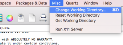
Figure 1. Screenshot of the macOS R.app console, selecting the Change Working Directory… option.

On Win11: File → Change dir…

Browse and select the folder in the same way you would for any app on your computer.

A second option is simply to tell R where to look using the setwd() function. Type the path or drag the folder/path into R

Example for macOS users:

#replace USERNAME with your user name. Replace BI311 with the name of your working folder
setwd("Users/USERNAME/Desktop/BI311/")

Example for Win11 users:

#replace USERNAME with your user name. Replace BI311 with the name of your working folder
setwd("C:/Users/USERNAME/Desktop")

Or, if you have not changed the backslash used in Win11 path to forward slash, the example was

setwd("C:\\Users\\USERNAME\\Desktop\\BI311")

On Win11 PCs, you can combine setwd() and choose.dir()

An advanced option is to nest the choose.dir() function within the call to set the working directory, like so

setwd(choose.dir())

which brings up a pop-up Explorer (Windows) from which you can select the directory (folder) you wish to use.

Again, this doesn’t work for macOS.

7. Access and use R GUI script window

Assuming you have pointed R to your working folder, create a new script document file. The following instructions show R GUI in a MacBook, but the instructions and view are similar in Windows PC.

From the R.app menu, select File > New Document (Fig 2).

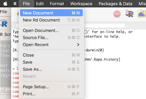
Figure 2. Screenshot of the macOS R.app console, selecting the New Document option.

The editor pops up with a text file (Fig 3).

Figure 3. Screenshot of the open script editor and macOS R.app console in the background.

Enter your script into the text area. When ready to run the script place the cursor at the line you wish to submit or highlight regions of code you wish to run. Then, press Command + return keys (Macs) or Ctrl + R key (Windows PC) to run the code (Fig 4).

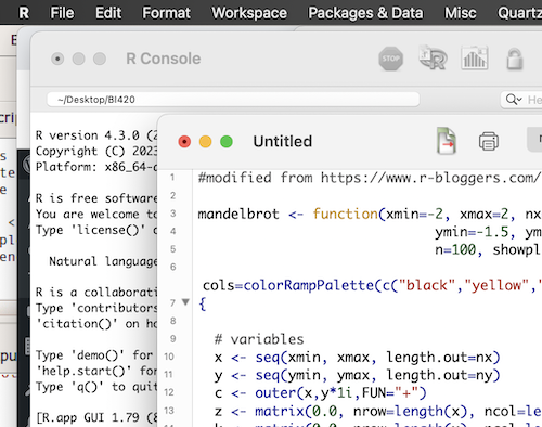
Figure 4. Screenshot of the script editor with a series of R commands. The macOS R.app console is in the background.

Don’t forget to save your coding work. From the text editor menu, File > Save as… (Fig 5).

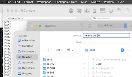
Figure 5. Screenshot file save as box in the script editor and macOS R.app console in the background.

8. R Commander windows

R Commander provides access to many statistical commands via drop down menus. The package provides a common user experience whether manOS or WinPC. R Commander is organized into four parts (Fig 6):

• Menus
• Script window
  • RMarkdown window (the second tab): See Part 09: Making a report
• Output window
• Messages window

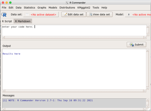
Figure 6. Screenshot of R Commander running on a WinPC.

Use menus to select Data to import and manage datasets, Statistics to Summarize (descriptive statistics), make inferences, or model data, Graphs provide access to several graph types, plus additional R commands.

The Script window can be used to enter commands directly (highlight one or more lines of code, press Submit button to run the code). R Commander will also print out the function calls made via Menus; this is a good way to learn how to code — R Commander generates the code based on menu choices, you then can go back and make changes to the code, adding color options, font size, etc., to refine your work.

We will rely on the script window in R Commander to carry out our work this semester. For more about the script window, see the Appendix: How to enter and run R code

Results from R commands are printed to the Output window. Graphs will popup as new windows. You may have to move around to find graph windows that may get hidden because we have several windows open on our desktops.

Error messages show up in red in Messages window. Error generates error reports when we have mistakes in our commands. Messages can start piling up; we can reset or clear the messages by clicking in the Message window, then selecting Rcmdr: Edit → Clear window.

9. Call system commands (optional)

CoLab, skip this step. Lastly, you can run simple commands on your computer, like checking files in a folder, while running R. Both macOS and Win11 has several 100 commands that can be entered through the terminal.

For example, on Win11, type and submit the following command in R

shell("dir /o")

and you’ll get a list of the files currently in your working folder.

On macOS, type and submit the following command in R

system("ls")

and you, too, will get a list of the files currently in your working folder.

Here’s another useful system command call from within R. Let’s say you want to check if our web site is running. One option is to ping the url letgen.org. Here’s how to do this in R running on Win11.

system2("ping",c("letgen.org"," -n 1"))

And R returns

Pinging letgen.org [50.87.81.216] with 32 bytes of data:
Reply from 50.87.81.216: bytes=32 time=86ms TTL=53

Ping statistics for 50.87.81.216:
Packets: Sent = 1, Received = 1, Lost = 0 (0% loss),
Approximate round trip times in milli-seconds:
Minimum = 86ms, Maximum = 86ms, Average = 86ms

On macOS

system2("ping",c("letgen.org"," -c 4"))

And R returns

PING letgen.org (50.87.81.216): 56 data bytes
64 bytes from from 50.87.81.216: icmp_seq=0 ttl=53 time=85.519 ms
64 bytes from from 50.87.81.216: icmp_seq=1 ttl=53 time=85.528 ms
64 bytes from from 50.87.81.216: icmp_seq=2 ttl=53 time=86.364 ms
64 bytes from from 50.87.81.216: icmp_seq=3 ttl=53 time=86.485 ms

--- letgen.org ping statistics ---
2 packets transmitted, 2 packets received, 0.0% packet loss
round-trip min/avg/max/stddev = 85.519/85.974/86.485/0.453 ms

Warning!

This next system command call can take a while on your computer — the command (systeminfo, system_profiler) is requesting a lot of information so the reply from your computer may take several seconds to complete.

And finally, you may need to get information about your computer. Rather than clicking through Win11 to get information, you can run an R command and save it to an R object like so.

myCPU <- system2("systeminfo", stdout=TRUE,stderr=TRUE,wait=TRUE); myCPU

and a long list about my Win11 computer will be stored in the object myCPU and displayed to the screen because I tagged on “;myCPU” at the end of the command. (Results not shown, it’s long).

On the macOS, one could repeat the above command, replacing “systeminfo” with “system_profiler“. However, I don’t recommend use of system_profiler (read further below) — instead for the macOS try sysctl .

I mentioned a warning. How long does systeminfo or system_profiler take? It’s going to depend on your computer, but if you’re curious, you can get the answer by wrapping the commands within an R function called system.time().

Here’s what the code would look like.

Win11

system.time(system2("systeminfo", stdout=TRUE,stderr=TRUE,wait=TRUE))

On my Win11 machine, the results were

 user system elapsed 
0.00    0.00    2.12

the elapsed time is the answer, 2.12 seconds.

On macOS

system.time(system2("system_profiler", stdout=TRUE,stderr=TRUE,wait=TRUE))

And on my macOS laptop, well, the spinning pinwheel flashed, then R crashed the second time I tried to run the system_profiler command. system_profiler is very, very thorough, returning much more information about your machine and software than you want to know.  In fairness to R, I was running several other apps at the same time (word processing and spreadsheet, networking software to share my screen, PowerPoint, Quicktime Player and several other apps). Just a reminder, best to shut down unnecessary apps. I shut down all other apps, restarted R and gave it another shot. Results were

  user system elapsed 
42.744 16.860  66.468

In conclusion, you CAN check system information, and on Win11 it is reasonable to do so within R. On macOS? Not recommended!

10. References & Suggested readings

11. Page quiz

Getting started

Seven questions from this page

Start Quiz

Question

Your answer:

Correct answer:

Next

Please wait..

↺

You got {{SCORE_CORRECT}} out of {{SCORE_TOTAL}}

Your Answers