Homework 10: Correlation and simple linear regression

Objectives:

• Explore null and alternate hypothesis concepts for coefficient estimates, linear association, and linear models.
• Evaluate error rates (Type I, Type II) and critical value, p-value.
• To compute how to obtain and interpret Product moment correlation and other correlations in R Commander
• To compute how to obtain and interpret  regression statistics and diagnostic plots in R Commander
• To apply General Linear Model approach to regression models

Homework 10 expectations

Read through the entire homework before starting to answer a question. You are expected to have read the chapter and to have completed preceding homework. Answers are provided to odd numbered problems — turn in your work for even numbered problems.

How to work this homework

This homework is in two parts and involves two separate data sets. First, Homework 9 asks you to practice R work on correlation. The data set is Animals, brain weight and body weight measured in grams for 28 mammals. Second, work with the data set cars, stopping distance by speed of the car, develop simple linear regression (SLR) models with diagnostic graphs.

Your report will consist of your answers to the bold, numbered questions (the even ones!) and supporting statistics from R. Suggested steps in your analysis are provided as numbered items (regular, not bold format). You may work together or individually, but each of your must turn in your own report. Don’t “plagiarize” from each other. Do include in your report who you worked with.

What to turn in: Turn in two properly named pdf files:

• CORR
• SLR

The pdfs file contain relevant R code, statistical results — edited to support your answers to the questions, and your answer to the questions (even numbered only). Use of RMarkdown recommended — because it is a simple way to include graphs generated; however copy/paste into a word document is also acceptable.

Submit your work to CANVAS. Obey proper file naming formats.

Resources for this homework

Chapter 16. Mike’s Biostatistics Book

Chapter 17. Mike’s Biostatistics Book

Mike’s Workbook for Biostatistics: A quick look at R and R Commander, Part01 – Part10 and previous homework pages presented in this workbook.

Additional R commands and or code provided below.

Answers to selected problems

Work on Correlation

Objective 1: To learn how to obtain and interpret Product moment correlation and other correlations in R Commander

Dataset

For correlation, use this dataset = Animals. This data set consists of brain weight and body mass of 28 species, including mammals (24 species plus humans) and three dinosaurs (Brachiosaurus, Dipliodocus, Triceratops). The ratio of brain weight to body mass (brain-body mass ratio) is related to the encephalization quotient (EQ); humans and other primates have a high ratio, so this measure is sometimes taken as a crude estimate of “intelligence.”

The data set is one of the built-in datasets with R, go to Rcmdr: Data in packages → Read data set from attached package… Select MASS package, then find Animals). Or, just load the data by submitting the code

data(Animals, package="MASS")

Alternatively, for your convenience, I’ve included the dataset at the end of this page (scroll down or click here).

Questions: The work to do for correlation analysis

1. Make a scatterplot of brain weight on body weight.

a) It would a good idea to highlight specific points in the graph.

classType <- c("M","M","M","M","M","D","M","M","M","M","M","M","M","H","M","D","M","M","M","M","M","M","M","M","M","M","D","M")
dAnimals <-data.frame(classType,Animals)
scatterplot(brain~body | classType, regLine=FALSE, smooth=FALSE, by.groups=TRUE, pch=c(19,19,19), cex=c(2,2,2), col=c("black", "blue", "red"), grid=FALSE, data=dAnimals)

2. Make histograms of body weight and brain weight

3. Conduct a test of normality of brain weight, and another test for body weight

Rcmdr: Statistics → Summaries → Test of normality (Compare Shapiro Wilks against Anderson-Darling)

R code

RcmdrMisc::normalityTest(~body, test="shapiro.test", data=Animals)

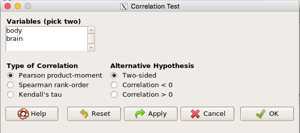
4. Obtain the Pearson product moment correlation (parametric) and conduct the two-sided test of the null hypothesis

Rcmdr: Statistics → Summaries → Correlation test

Figure 1. Screenshot correlation test R Commander menu

R code

cor.test(Animalsbrain, alternative="two.sided", method="pearson")

4a. Find in the R output the command for correlation and make sure you include this in your report.

5. Repeat, but this time calculate the (nonparametric) Spearman rank-order correlation, again a two-sided test

5a. Find in the R output the command for Spearman rank-order correlation and make sure you include this in your report.

Question 1. Briefly define and contrast parametric and nonparametric statistical tests. (Hint: assumptions!)

Question 2. Make a preliminary conclusion about whether or not brain weight is correlated with body weight.

Question 3. Using the results from items 2 – 5, which correlation estimate is most justifiable as a test of the association between brain and body weight, the parametric or the nonparametric correlation?

Question 4. Reviewing your plot and the correlation results, comment on the relationship between body mass and brain weight.

Save your Markdown file and include Corr as part of your properly named pdf file name. Submit your file to this page.

Proceed to the second part of the homework

Work on Ordinary Linear (Simple) Regression

Objective 2: To learn how to obtain and interpret regression statistics and diagnostic plots in R Commander

Objective 3: To compare models and evaluate “best fit,” with use of R2, the coefficient of determination.

Objective 4: Introduce the General Linear Model approach

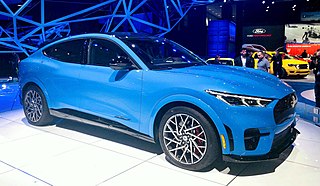
For simple linear regression use this dataset = cars, Speed and Stopping Distances of Cars (one of the built-in datasets with R, go to Rcmdr: Data in packages → Read data set from attached package… Select datasets package, then find cars). More simply, at the R prompt write and submit

data(cars, package="datasets")

Alternatively, and for your convenience, I’ve included the dataset at the end of this page (scroll down or click here). The data set is a classic from the 1920s; it’s about distance (feet) to stop a car by speed (mph) of a car (see Wikipedia). Thus, the cars in 1920s looked more like the one on left than the one at right (Fig 2).

Wikipedia, CC BY-SA 4.0

Wikipedia, CC BY-SA 4.0

Figure 2. The stopping distance  data set is an old one — data from a car similar to the Ford Model A at left, not the Ford Mustang Mach E GT at right.

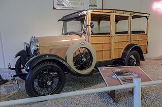
The work to do on simple linear regression

1. Identify the dependent and independent variables. Justify your selection

2. Make a scatterplot of Distance on Speed

3. Make a histogram of Distance

4. Conduct a test of normality on Distance

Rcmdr: Statistics → Summaries → Test of normality (Compare Shapiro Wilks against Anderson-Darling)

Question 1. Make a preliminary conclusion about whether or not the data conforms to assumptions of linear regression based on your results from items 1 – 4. Include your justification for choice of independent and dependent variables. If you find the data do not conform, create new log-transformed, log10(), variables and redo your assumption tests.

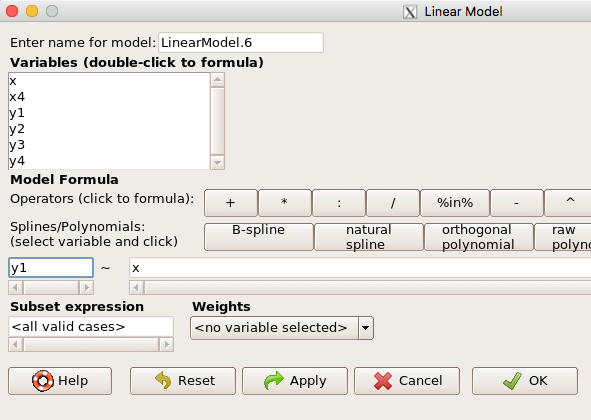
5. Based on your answer to Question 1, write out the model, e.g., in R, the model is specified as Y ~ X, then go ahead and conduct the linear regression of Distance and Speed.

Rcmdr: Statistics → Fit models → Linear model

• an example screen is shown (yours will look different from the example). Note also that you can let Rcmdr assign a name for the model object or you can specify one yourself (⮜ DrD recommended!)

Figure 3. Screenshot linear regression menu R Commander.

R code

RegModel.1 <- lm(dist~speed, data=cars)
summary(RegModel.1)

6. Obtain the following from the R output ⮜ recommend you organize these into a table

a) value of the Y-intercept

b) Report on whether the Y-intercept is statistically significant (what is the null hypothesis?)

c) value of the slope

d) Report on whether the slope is statistically significant (what is the null hypothesis?)

e) Write out the statistical model

f) Find the fit statistic for this model.

Question 2. Make a preliminary conclusion about the predictive value of your X (independent) on your Y (dependent) variable

7. Repeat steps 5 and 6, but for the untransformed response variable (– or, if you used the raw, untransformed response variable previously, now run the regression with the transformed variable).

a) record the linear model

b) record the fit statistics (R2 and RSE).

c) compare fit of regressions of the transformed vs untransformed variables. Which is best?

8. Obtain appropriate diagnostic plots and diagnostic statistics for your regression and evaluate your model(s) against the assumptions

Rcmdr: Models → Graphs → Basic diagnostic plots

R code

plot(RegModel.1)

Rcmdr: Models → Numerical diagnostics → “several to choose from” ⮜ part of the evaluation is whether you select the correct diagnostic tests; hint: most of these are listed in your Chapter 18)

R code example, RESET test for nonlinearity

resettest(dist ~ speed, power=2:3, type="regressor", data=cars)

Question 3. Make a conclusion about the regression model based on your results from Question 1 and Question 2.

Question 4. Use your regression model to predict stopping distance at 60 mph. How does your prediction compare to stopping distance of 108 feet for a Ford Mustang at the same speed?

Hint: you can simply calculate this using the appropriate numbers from your regression model. Instead of “hand” calculations, alternatively, you could use the following command

predict(modelName, data.frame(nameOfdependent=c(60)))

where modelName is replaced with the object name for your regression model, and nameOfdependent is replaced with the name of your independent variable.

Regardless of method you choose, if you used log-transform, then don’t forget to report your predicted value in original raw form. For example, if log(x, 10), then the anti-log 10^x, with x equal to your predicted value. This is a standard recommendation for data analysis — do your statistics on the transformed data, but for graphics or other reports, always back-transform the data.

Save your Markdown file and include SLR as part of your properly named pdf file name. Submit your file to this page.

This concludes work for Homework 10

Bonus

Jerison’s EQ was calculated as

Calculate EQ for chimpanzee, elephant, human, mouse in the Animal data set.

R or Rcmdr commands

myData <- read.table(header=TRUE, sep="\t", text = "
insert your data table here
")

head(myData)

Test normality.

Rcmdr → Statistics → Summaries → Test for normality

Other R/Rcmdr commands provided in text

Data

Dataset = Animals from R package MASS

Dataset = cars

/MD